Optimizing Resource Efficiency in Large-Scale Systems

Analyzing Resource Usage at Scale

The first rule of optimization is that you cannot improve what you cannot measure. In a distributed environment with tens of thousands of machines running millions of tasks, "measuring" is a formidable data engineering challenge. You need a system that can continuously collect detailed performance data from every corner of the fleet with negligible overhead.

Google's solution to this is a system called Google-Wide Profiling (GWP). It provides the foundational data for almost all large-scale efficiency analysis.

As the paper highlights, GWP's genius lies in its two-dimensional sampling strategy: it profiles only a small, random subset of machines at any given time, and on those machines, it uses standard event-based sampling. This combination keeps the fleet-wide overhead below 0.01% while still collecting a statistically representative dataset.

This rich dataset allows engineers to answer critical efficiency questions:

• What are the most CPU-intensive functions across the entire fleet? (As the paper notes, this identified zlib as consuming 5% of all cycles, motivating a company-wide optimization effort).
• Which applications are "memory hogs"?
• How does the performance of an application differ across software versions or hardware platforms?

This continuous, fleet-wide view is the starting point for all major efficiency improvements.

Strategies for Improving Resource Efficiency

Once you can accurately measure resource consumption, you can begin to optimize it. At Google, this is primarily achieved through the cluster manager, Borg. Let's explore the key strategies it employs, many of which have direct counterparts in its open-source successor, Kubernetes.

A 2020 paper analyzing a decade of Borg's evolution provides incredible insights into this.

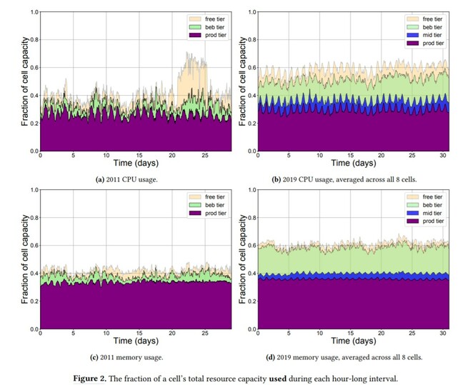
Strategy 1: Statistical Multiplexing and Overcommitment

The most significant efficiency gain comes from a simple observation: most jobs don't use all the resources they request. This gap between the requested limit and the actual usage is called "slack."

There are valid reasons users over-request resources, as John Wilkes explains in his talk on Borg.

Borg turns this "wasteful" slack into a massive efficiency win by using it to run low-priority, non-latency-sensitive "best-effort batch" jobs. Production jobs get a reservation based on their recent usage, which Borg guarantees. The space between this reservation and their padded limit is then "reclaimed" and offered to batch jobs.

This policy of co-locating production and batch workloads has a staggering economic impact.

A 25% reduction in the size of Google's fleet represents a multi-billion dollar saving. This is a clear example of how a technical decision in system design directly drives business value.

The "Borg: the Next Generation" paper provides the data to back this up.

Strategy 2: Fine-Grained and Automated Resource Allocation

Another source of inefficiency is "internal fragmentation" caused by rigid resource allocation units.

• Fine-Grained Requests: Many cloud platforms offer fixed T-shirt sizes (small, medium, large VMs). If your job needs 2.1 cores, you have to request 4, wasting 1.9 cores. Borg avoids this by allowing users to request resources with high precision (e.g., to the millicore or byte). Wilkes' talk reveals that forcing power-of-two rounding would require 30% more machines (cost of rounding up in resource LINK). This is the motivation behind Google Cloud's custom machine types.

• Automated Vertical Scaling: Even with fine-grained requests, asking developers to perfectly specify them is unrealistic. To solve this, Google developed Autopilot, a system that automatically adjusts a task's resource limits based on its historical and current usage.

Strategy 3: Affinity-Based Scheduling

The most sophisticated schedulers go beyond simple bin-packing of resource quantities and consider the affinity between workloads and hardware.

• CPU Affinity: An application's code may run more or less efficiently (measured in Cycles Per Instruction, or CPI) on different processor microarchitectures. The GWP paper you read earlier describes how profiling data can be used to measure this. A smart scheduler can use this data to place jobs on the hardware where they run fastest, improving overall throughput. The paper estimates this could yield a 10-15% improvement in fleet-wide efficiency.

• Network Affinity: In our previous lesson, we discussed how Borg can perform hotspot-aware task placement to avoid overwhelming Top-of-Rack network switches. This is another form of affinity scheduling, where the scheduler considers network topology and utilization to improve network efficiency. At an even more advanced level, Google's datacenter fabric itself can be reconfigured.

This ability to dynamically re-wire the network based on observed traffic patterns is a powerful tool for maximizing network efficiency, ensuring that bandwidth is allocated where it's most needed.

The Challenge of "Hogs and Mice"

A final, crucial insight from the analysis of Google's workload is its extremely heavy-tailed nature.

The key finding is that the top 1% of jobs ("hogs") consume over 99% of all resources. The remaining 99% of jobs ("mice") use a tiny fraction. From queueing theory, we know that systems with high service time variance (a high squared coefficient of variation, or $C^2$) suffer from long queueing delays, as small jobs get stuck behind large ones. The paper notes that Google's workload has an incredibly high $C^2$ of over 23,000.

This implies that a critical strategy for both efficiency and performance is to design schedulers that can isolate the "mice" from the "hogs," allowing the vast majority of jobs to run in what feels like a very lightly loaded system.

A Systems View of Performance Engineering

While we've focused on Google's specific solutions, the underlying principles are universal. A talk from a performance engineer at Twitter provides an excellent framework for thinking about this problem more broadly.

This perspective reinforces everything we've seen: effective resource management begins with building a model of your system, establishing a comprehensive data collection pipeline (like GWP), and then performing analysis—a "counting exercise"—on that data to drive optimization. The mention of using eBPF for low-overhead, high-granularity data collection is a nod to the modern tooling used for this purpose at many large tech companies.

Conclusion

In this lesson, we moved from the tactical problem of hotspot mitigation to the strategic challenge of fleet-wide resource efficiency. You've seen that at Google's scale, efficiency is not an afterthought but a central design driver, saving billions of dollars and enabling more work to be done with the same physical hardware.

Your key takeaways are:

• Analysis is paramount: You can't optimize what you can't measure. Systems like Google-Wide Profiling provide the continuous, low-overhead, fleet-wide data needed to identify inefficiencies.
• Reclaim all waste: The largest efficiency gains come from statistical multiplexing—reclaiming the "slack" between requested and used resources to run lower-priority workloads.
• Allocation matters: Efficiency is improved by avoiding fragmentation through fine-grained resource requests and by automating resource allocation with tools like Autopilot to eliminate human error and guesswork.
• Be affinity-aware: The best schedulers consider the affinity between workloads and hardware (both CPU and network) to maximize throughput.
• Isolate hogs from mice: Recognizing and managing the heavy-tailed nature of workloads is critical for ensuring that the vast majority of small jobs see good performance.

In our next lesson, we will build on this foundation. We will learn how to formulate a capacity plan for a distributed system considering growth forecasts and SLOs. Now that you understand how to measure and maximize the efficiency of your current resources, the next logical step is to predict how many resources you'll need in the future.