Thévenin's Theorem for DC Circuit Simplification

Why We Need an Equivalent Circuit

Imagine you're designing a system where you need to test how different sensor modules (the "load") behave when connected to your main circuit. As we saw with the voltage divider, each time you swap the load resistor $R_L$, the overall circuit's properties change, forcing a complete re-analysis. This is tedious and impractical.

Thévenin's theorem offers a brilliant solution. It allows us to characterize the rest of the circuit—everything except the load—by asking: "From the load's perspective, what does this circuit look like?" The answer is always the same: it looks like an ideal voltage source ($V_{th}$) with a single resistor in series ($R_{th}$). Once you find these two values, you can analyze the load's behavior for any $R_L$ by solving a simple series circuit, dramatically simplifying your work.

The Thévenin Equivalent Circuit

Thévenin's theorem states that any linear two-terminal circuit can be replaced by an equivalent circuit consisting of a single voltage source, $V_{th}$, in series with a single resistor, $R_{th}$.

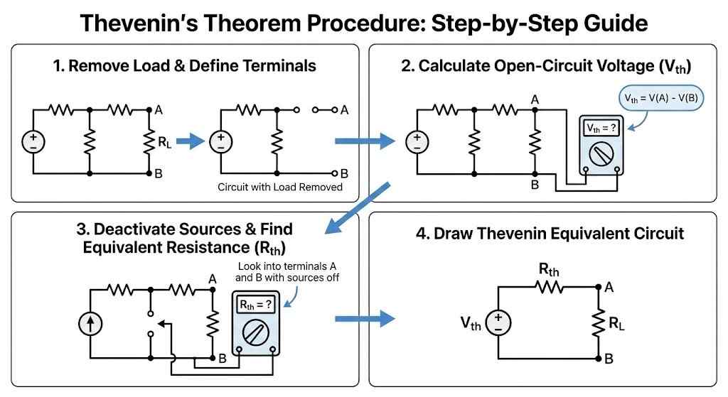
To create this equivalent circuit, we need to find two values: the Thévenin Voltage ($V_{th}$) and the Thévenin Resistance ($R_{th}$). The process is a systematic, two-step procedure.

Step 1: Finding the Thévenin Voltage ($V_{th}$)

The Thévenin voltage is the open-circuit voltage at the terminals where the load is connected.

Procedure:

1. Remove the load resistor from the circuit, leaving the terminals (let's call them A and B) open.
2. Calculate the voltage across these open terminals, $V_{AB}$. This voltage is your Thévenin voltage, $V_{th}$.

Because no current can flow out of the open terminals, this calculation is often simpler than analyzing the original, fully connected circuit. You can use any of your known analysis techniques, like Ohm's Law, KVL, or the voltage divider rule.

Step 2: Finding the Thévenin Resistance ($R_{th}$)

The Thévenin resistance is the equivalent resistance of the circuit "looking back" into the terminals where the load was connected, with all independent sources deactivated.

Procedure:

1. Remove the load resistor (if you haven't already).
2. Deactivate all independent sources:
   • Voltage sources are replaced with short circuits (a wire with zero resistance).
   • Current sources are replaced with open circuits (a break in the wire).
3. Calculate the equivalent resistance between the terminals A and B. This is your Thévenin resistance, $R_{th}$.

Why do we do this? An ideal voltage source maintains a constant voltage regardless of current; its internal resistance is zero. Setting its voltage to zero makes it behave like a perfect wire (a short). An ideal current source provides a constant current regardless of voltage; its internal resistance is infinite. Setting its current to zero makes it behave like a break in the circuit (an open).

This step requires a crucial shift in perspective. You are no longer looking at the resistance from the source's point of view, but from the load's.

A Worked Example

Let's apply this full procedure to a slightly more complex circuit. This will solidify the steps and highlight the importance of careful node identification.

We will follow the six-step process outlined in the following video to analyze a circuit.

Let's break down the analysis from the video's second example.

The Circuit:

• A 100V source connected to a 10Ω resistor.
• An 80V source connected to a 20Ω resistor.
• The 10Ω and 20Ω resistors are connected at a common node, 'A'.
• The other sides of the sources are connected to a common ground, node 'B'.
• A 50Ω load resistor is connected between nodes A and B.

1. Find $R_{th}$:

• Remove the 50Ω load resistor.
• Deactivate the sources: replace the 100V and 80V sources with short circuits.
• With both sources shorted, the 10Ω and 20Ω resistors are now connected between node A and the common ground (node B). This means they are in parallel.
• Calculate the equivalent resistance: $$R_{th}=R_1||R_2=\frac{10\times 20}{10+20}=\frac{200}{30}\approx 6.67\Omega$$

2. Find $V_{th}$:

• Keep the load resistor removed. The original sources are active.
• The 100V source, 10Ω resistor, and 20Ω resistor, and 80V source now form a single series loop. Note the sources oppose each other.
• First, find the current flowing in this loop using KVL: $$100V-I(10\Omega )-I(20\Omega )-80V=0$$ $$20V=I(30\Omega )⟹I=\frac{20V}{30\Omega }\approx 0.667A$$
• The Thévenin voltage $V_{th}$ is the voltage at node A relative to node B (ground). We can find this by starting at the 100V source and subtracting the voltage drop across the 10Ω resistor: $$V_{th}=V_A=100V-(I\times 10\Omega )=100V-(0.667A\times 10\Omega )=100V-6.67V\approx 93.33V$$

3. Draw the Equivalent Circuit and Analyze the Load:

• The entire complex network is now replaced by a 93.33V source ($V_{th}$) in series with a 6.67Ω resistor ($R_{th}$).
• We can now re-connect our 50Ω load resistor and easily find the voltage across it using the voltage divider rule on this new, simple circuit: $$V_L=V_{th}\times \frac{R_L}{R_{th}+R_L}=93.33V\times \frac{50\Omega }{6.67\Omega +50\Omega }\approx 82.3V$$

This final calculation is far simpler than performing a mesh or nodal analysis on the original circuit.

The Practical Meaning of $V_{th}$ and $R_{th}$

Now that you understand the mechanics, let's circle back to the practical implication. The Thévenin equivalent provides a perfect model for the "loading effect" we discussed in the last lesson.

• $V_{th}$ is the ideal, open-circuit (unloaded) voltage of the circuit at its output terminals.
• $R_{th}$ is the circuit's effective output resistance. It's this resistance that causes the voltage to drop when a load draws current. The voltage drop is simply $I_L\times R_{th}$.

This framework is not just a calculation trick; it's a fundamental concept for characterizing the output of any circuit block, from a simple voltage divider to a complex amplifier or power supply.

Conclusion

Today, you've learned one of the most powerful simplification techniques in circuit analysis. By abstracting a complex linear network into a simple equivalent, Thévenin's theorem allows you to efficiently analyze how a circuit interacts with different loads.

Key Takeaways:

• Thévenin's Theorem simplifies any linear two-terminal circuit into an equivalent circuit with a single voltage source ($V_{th}$) and a single series resistor ($R_{th}$).
• $V_{th}$ is the open-circuit voltage at the terminals of interest (load removed).
• $R_{th}$ is the equivalent resistance at the terminals, with all independent voltage sources shorted and all independent current sources opened.
• This equivalent circuit provides a practical model for a circuit's output, where $V_{th}$ is the ideal output voltage and $R_{th}$ is the output resistance responsible for voltage drop under load.

In our next lesson, we will begin our journey into practical, hands-on electronics by learning to use a multimeter. You will see how we can use this essential tool to physically measure voltage, current, and resistance, allowing us to experimentally verify the $V_{th}$ and $R_{th}$ values we've learned to calculate today.