NumPy Linear Algebra Fundamentals

Introduction

In our last lesson, you did an excellent job implementing fundamental vector and matrix operations from scratch. That exercise was crucial for building a deep, first-principles understanding of how these operations work. You likely noticed, however, that the pure Python implementations were verbose and, for larger matrices, would not be very performant.

Today, we transition from "how it works" to "how it's done in practice." Our learning outcome is to perform fundamental linear algebra operations—specifically matrix multiplication, inversion, and eigendecomposition—using NumPy. NumPy is the cornerstone of the scientific computing stack in Python, providing highly optimized data structures and routines for numerical operations. This lesson will bridge your foundational knowledge with the practical tools you'll use throughout your computer vision journey.

Let's get started.

From Python Lists to NumPy Arrays

First, we need to introduce NumPy's core data structure: the ndarray (n-dimensional array). Unlike Python lists, which are flexible but slow, NumPy arrays are dense, fixed-type arrays of elements. This homogeneity allows NumPy to perform operations using highly optimized, pre-compiled C or Fortran code, leading to massive performance gains.

You can create arrays from Python lists. A list of numbers becomes a 1D array (a vector), and a list of lists becomes a 2D array (a matrix).

import numpy as np

# Creating a vector (1D array)
py_vector = [1, 2, 3]
np_vector = np.array(py_vector)
print(f"NumPy vector:\n{np_vector}")

# Creating a matrix (2D array)
py_matrix = [[1, 2], [3, 4]]
np_matrix = np.array(py_matrix)
print(f"\nNumPy matrix:\n{np_matrix}")

# You can check the dimensions using the .shape attribute
print(f"\nShape of the matrix: {np_matrix.shape}") # Output: (2, 2)

Basic Matrix Operations with NumPy

Let's revisit the operations we built from scratch and see how elegantly NumPy handles them. The following resource provides a comprehensive guide with code examples that we will follow.

As you've just read, the syntax is incredibly intuitive:

• Addition and Scalar Multiplication: These use the standard + and * operators, just like with regular numbers.

  A = np.array([[1, 2], [3, 4]])
  B = np.array([[5, 6], [7, 8]])
  
  # Addition
  print("A + B:\n", A + B)
  
  # Scalar multiplication
  print("\n2 * A:\n", 2 * A)
  

• Transpose: You can transpose a matrix using the .T attribute.

  A = np.array([[1, 2, 3], [4, 5, 6]])
  print("A.T:\n", A.T)
  

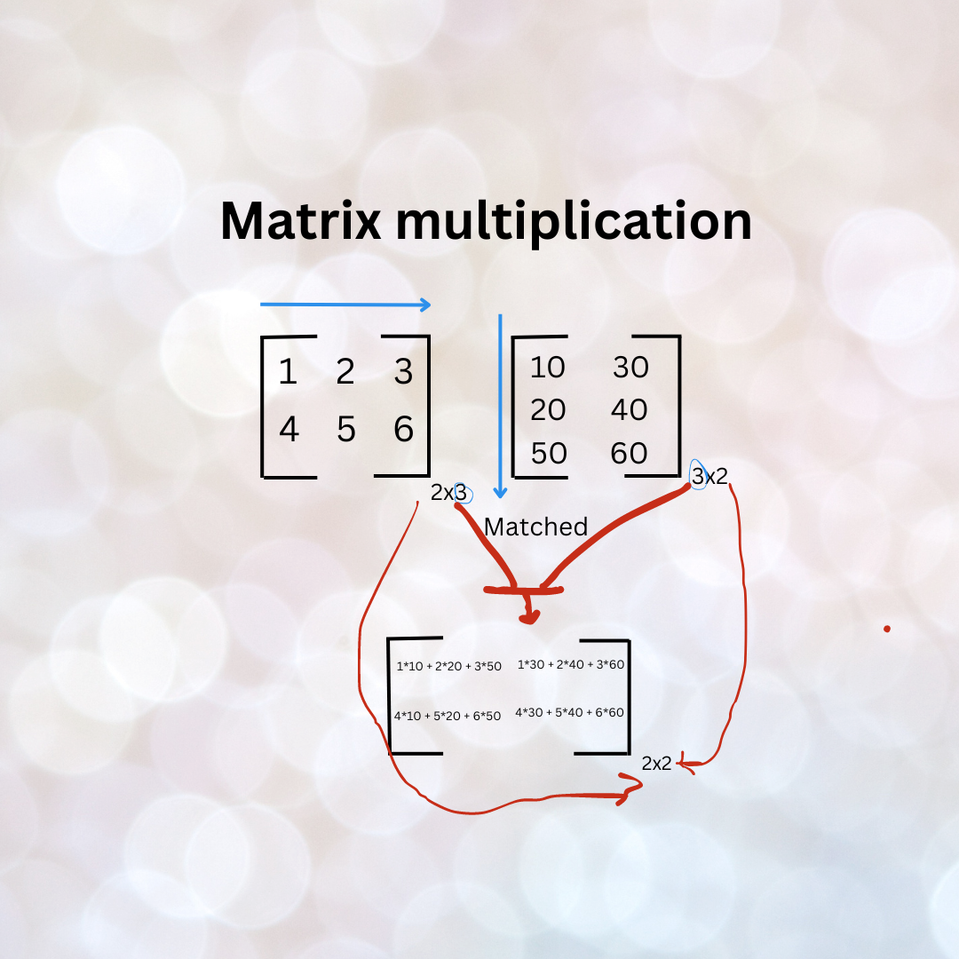
• Matrix Multiplication: This is a critical operation with a specific operator. In Python 3.5+, the @ operator was introduced for matrix multiplication. It is the modern, recommended way. The np.dot() function does the same thing.

  • Crucial Distinction: The * operator performs element-wise multiplication (also known as the Hadamard product), not matrix multiplication. This is a very common source of bugs.

  A = np.array([[1, 2], [3, 4]])
  B = np.array([[5, 6], [7, 8]])
  
  # Matrix multiplication
  print("A @ B:\n", A @ B)
  
  # Element-wise multiplication (Hadamard product)
  print("\nA * B:\n", A * B)
  

  The operation A @ B performs the series of dot products between rows of A and columns of B, just as we implemented manually.

Matrix Inversion

The inverse of a square matrix $A$, denoted $A^{-1}$, is the matrix that, when multiplied by $A$, yields the identity matrix $I$. It's conceptually similar to the reciprocal of a number (e.g., $5\times 5^{-1}=1$).

The inverse is fundamental for solving systems of linear equations of the form $Ax=b$. If $A$ is invertible, we can find $x$ by computing $x=A^{-1}b$.

To compute the inverse, we use the np.linalg.inv() function from NumPy's linear algebra submodule.

# A must be a square matrix
A = np.array([[1, 3], [2, 2]])

# Check if it's invertible by checking if the determinant is non-zero
determinant = np.linalg.det(A)
print(f"Determinant of A: {determinant:.2f}")

if determinant != 0:
    A_inv = np.linalg.inv(A)
    print(f"\nInverse of A:\n{A_inv}")

    # Verify that A @ A_inv gives the identity matrix
    # np.eye(n) creates an n x n identity matrix
    identity = A @ A_inv
    print(f"\nA @ A_inv:\n{np.round(identity, 5)}") # Round to handle tiny floating point errors
else:
    print("\nMatrix A is singular and cannot be inverted.")

A Better Way to Solve Linear Systems

While you can solve $Ax=b$ by finding the inverse and computing x = np.linalg.inv(A) @ b, it is not the recommended approach. Calculating the inverse is computationally expensive and can be numerically unstable. A more direct and robust method is to use np.linalg.solve().

The np.linalg.solve(A, b) function solves the system $Ax=b$ without explicitly computing the inverse, typically using a more stable method like LU decomposition, which is a direct outcome of the Gaussian elimination process you just read about.

# Solve the system Ax = b
# A = [[1, 3], [2, 2]]
# b = [[-1], [1]]

A = np.array([[1, 3], [2, 2]])
b = np.array([[-1], [1]])

# Solve using the numerically preferred method
x = np.linalg.solve(A, b)

print(f"Solution x:\n{x}")

# Verification: A @ x should equal b
print(f"\nVerification (A @ x):\n{A @ x}")

Eigendecomposition

Finally, let's tackle eigendecomposition. As a refresher, for a given matrix $A$, an eigenvector $v$ and its corresponding eigenvalue $\lambda$ satisfy the equation $Av=\lambda v$. Eigendecomposition is the process of breaking a matrix down into its constituent eigenvalues and eigenvectors, expressed as $A=X\Lambda X^{-1}$, where $X$ is the matrix of eigenvectors and $\Lambda$ is the diagonal matrix of eigenvalues.

This decomposition is a cornerstone of many machine learning algorithms, including Principal Component Analysis (PCA), which you will encounter later.

NumPy's np.linalg.eig() function makes this process straightforward.

A = np.array([[4, 2], [1, 3]])

# Compute eigenvalues and eigenvectors
eigenvalues, eigenvectors = np.linalg.eig(A)

print(f"Eigenvalues:\n{eigenvalues}")
print(f"\nEigenvectors (each column is an eigenvector):\n{eigenvectors}")

# Let's verify the Av = λv property for the first eigenvalue/eigenvector pair
lambda1 = eigenvalues[0]
v1 = eigenvectors[:, 0] # Get the first column

print(f"\n--- Verification for first pair ---")
print(f"A @ v1 = {A @ v1}")
print(f"lambda1 * v1 = {lambda1 * v1}")
print(f"Are they close? {np.allclose(A @ v1, lambda1 * v1)}")

# Now, let's reconstruct A from its eigendecomposition: A = XΛX⁻¹
X = eigenvectors
Lambda = np.diag(eigenvalues) # Create a diagonal matrix from eigenvalues
X_inv = np.linalg.inv(X)

A_reconstructed = X @ Lambda @ X_inv

print("\n--- Reconstruction ---")
print(f"Original matrix A:\n{A}")
print(f"\nReconstructed matrix A:\n{A_reconstructed}")
print(f"\nDo they match? {np.allclose(A, A_reconstructed)}")

M = np.array([[2, 1], [1, 2]])
y = np.array([4, 5])

import numpy as np

M = np.array([[2, 1], [1, 2]])
y = np.array([4, 5])

# 1. Calculate the inverse
M_inv = np.linalg.inv(M)
print(f"1. Inverse of M:\n{M_inv}\n")

# 2. Solve Mx = y
x = np.linalg.solve(M, y)
print(f"2. Solution for x:\n{x}\n")
# You can verify this: M @ x gives [4. 5.]

# 3. Eigendecomposition
eigenvalues, eigenvectors = np.linalg.eig(M)
print(f"3. Eigenvalues:\n{eigenvalues}")
print(f"   Eigenvectors:\n{eigenvectors}\n")

# 4. Reconstruct M
X = eigenvectors
Lambda = np.diag(eigenvalues)
X_inv = np.linalg.inv(X)
M_reconstructed = X @ Lambda @ X_inv
print(f"4. Reconstructed M:\n{M_reconstructed}")
print(f"   Matches original? {np.allclose(M, M_reconstructed)}")

Conclusion

This lesson marks the end of our foundational module on linear algebra. You have progressed from understanding the abstract concepts, to implementing them from scratch, and now to using the industry-standard tool, NumPy, to perform these operations efficiently.

Key Takeaways:

• NumPy's ndarray is the fundamental object for numerical computation in Python.
• Basic operations like addition, scalar multiplication, and transposition have simple, intuitive syntax (+, *, .T).
• Matrix multiplication is performed with the @ operator, while * performs element-wise multiplication.
• The inverse of a matrix is found with np.linalg.inv(), but np.linalg.solve() is the preferred, more stable method for solving linear systems.
• Eigendecomposition is performed with np.linalg.eig(), which returns both eigenvalues and eigenvectors, allowing you to analyze and reconstruct matrices.

Preview of the Next Lesson:

With a solid grasp of linear algebra, we are now ready to tackle the second mathematical pillar of machine learning: calculus. In the next module, we will explore how calculus provides the tools for optimization, which is at the heart of training almost every machine learning model. We will begin by deriving the concept of the derivative from first principles, understanding it as a measure of instantaneous rate of change.