Introduction
In our last two lessons, we built the foundation for a data-driven coaching practice. We started with designing single-case experiments (SCEDs) to test your interventions and then developed the customized tracking tools (using EMA principles) needed to collect the data for those experiments. You now have a framework for setting up an experiment (Phase A baseline, Phase B intervention) and a method for gathering client data in real-time. The question that naturally follows is: what do you do with that data as it streams in?
This lesson directly addresses the learning outcome: Apply Bayesian reasoning to conceptually update beliefs about intervention effectiveness as new client data comes in. Given your background in Bayesian Decision Theory, you're already familiar with the mathematical underpinnings. Our focus today will not be on re-deriving Bayes' theorem, but on applying it as a powerful conceptual model for coaching. We will frame it as a formal system for doing what great coaches do intuitively: updating their assessment of what works for a client based on new observations.
The Bayesian Mindset: From "Is it True?" to "How Sure Am I?"
The frequentist approach, often associated with the kinds of experiments we discussed (like A-B testing), typically seeks a binary answer at the end of a study: was the intervention effective, yes or no (reject or fail to reject the null hypothesis)? The Bayesian approach offers a different, and for coaching, often more useful perspective. It's not about waiting until the end to pass judgment; it's about continuously updating your degree of belief.
This short video from the New England Journal of Medicine provides an excellent conceptual overview of this shift in thinking.
This video contrasts the frequentist and Bayesian paradigms using a simple, relatable example.
Pay close attention to the fundamental difference in how the two approaches treat data and parameters. Then, focus on the explanation of how a prior distribution (your initial belief) is updated by data to form a posterior distribution (your new, more informed belief). The walkthrough of the commuter example beautifully illustrates how this provides more nuanced insights than a simple "yes/no" answer.
As the video illustrates, Bayesian inference is built on three core components. Let's formally define them in the context of your coaching practice.
Bayesian evaluation of behavior change interventions - PMC - NIH
This paper provides a clear, non-mathematical introduction to the three pillars of Bayesian inference, using helpful visuals. It's a great refresher on the core logic.
Start with the section on "Bayesian inference." The authors' goal here is to build a visual intuition, which is perfect for our purposes. Read the subsections explaining the role of each of the three components: The Prior: This represents your belief about an intervention's effectiveness before you see any new data from this specific client. It's your professional hypothesis, informed by theory, past clients, and the intake data. The Likelihood: This is the new information—the data you collect with your repeated-measures tracking tool. The Posterior: This is your updated belief, the result of combining your prior with the new data. The figures in this section (Figures 1, 2, and 3) do a great job of showing how the prior and likelihood combine to create the posterior. The posterior is essentially a compromise between what you initially believed and what the new evidence suggests.
The Bayesian Workflow for Coaching
This process of updating beliefs isn't a one-time event; it's a continuous cycle. As a coach, you are constantly refining your understanding of a client. The Bayesian workflow provides a structure for this process.

Let's walk through this workflow, adapting it into a practical protocol for your consulting engagements.
1. Define Priors (Set Your Hypothesis)
Before implementing a new coaching strategy, you formalize your initial belief. This is your prior distribution. For you, this isn't just a vague hunch; it's an educated guess based on your expertise.
- Parameter of Interest (): This is the effect you're trying to measure. For example, could be the "average daily change in a client's compersion score" after you introduce a new journaling exercise.
- Specifying the Prior: You don't need to write complex equations. You can state it qualitatively: "My prior belief is that this journaling exercise will have a small to medium positive effect on compersion. There is a small chance it has no effect, and a very small chance it could backfire and increase jealousy."
This practice of explicitly stating your initial beliefs is a cornerstone of a rigorous, scientific approach. A key is to use weakly informative priors—priors that rule out absurdities (e.g., a 1000% increase in satisfaction) but are broad enough to let the client's data drive the conclusion.
Practical Bayesian Inference in Astronomy - Andy Casey
This guide for astronomers gives outstanding, field-agnostic advice on the practicalities of choosing priors. The principles of avoiding "vacuous" or "restrictive" priors are universal.
Read the subsection "A Taxonomy of Priors" and the following "The Two Failure Modes of Prior Specification." This will reinforce the goal of setting a prior that is informed but not so rigid that it ignores the data.
2. Collect Data (The Likelihood)
Your client engages with the intervention and uses the EMA tracking tool you designed in the previous lesson. Each new data point (e.g., a daily compersion score, a log of time spent on lifestyle logistics) contributes to the likelihood. This is the evidence that will challenge or support your prior belief.
3. Update Beliefs (Calculate the Posterior)
This is the heart of the process. The posterior distribution of your belief becomes the prior distribution for the next piece of data you collect. This is known as sequential updating.
Posterior(Today) ∝ Likelihood(Today's Data) × Prior(Yesterday's Posterior)
Imagine you see two consecutive days of increased compersion scores. Your belief in the intervention's effectiveness strengthens. If you see two days of decreased scores, your belief weakens. This iterative process is what makes Bayesian reasoning so powerful for N-of-1 analysis like coaching.
Practical Bayesian Inference in Astronomy - Andy Casey
This short section perfectly captures the mechanism of iterative learning.
Read the subsection "Sequential updating in practice". The example of analyzing data in two batches is exactly analogous to you analyzing client data as it comes in day by day or week by week. The final posterior is the same as if you'd analyzed all the data at once, but the process allows for real-time insight.
4. Check Your Model (Posterior Predictive Checks)
Once you have an updated belief (a posterior), you need to check if it's a good belief. In statistics, this is called model checking. A key technique is the Posterior Predictive Check (PPC).
The question a PPC asks is: "If my new belief about the intervention's effectiveness is correct, what kind of data would I expect to see? And does the data I've actually seen look like that?"
- Example: Your posterior belief is that the journaling exercise has a strong, stable, positive effect. But the client's actual data shows wild swings—high one day, low the next. Your model fails the check. The data is telling you your belief is too simplistic. Perhaps the intervention works, but its effect is moderated by another factor (e.g., it only works on days the client gets enough sleep). This tells you where to investigate next.
This step prevents you from becoming overconfident in a flawed hypothesis and forces you to confront discrepancies between your theory and the client's reality.
A Concrete Example: Analyzing George's Data
Let's apply this workflow to a single-case dataset.
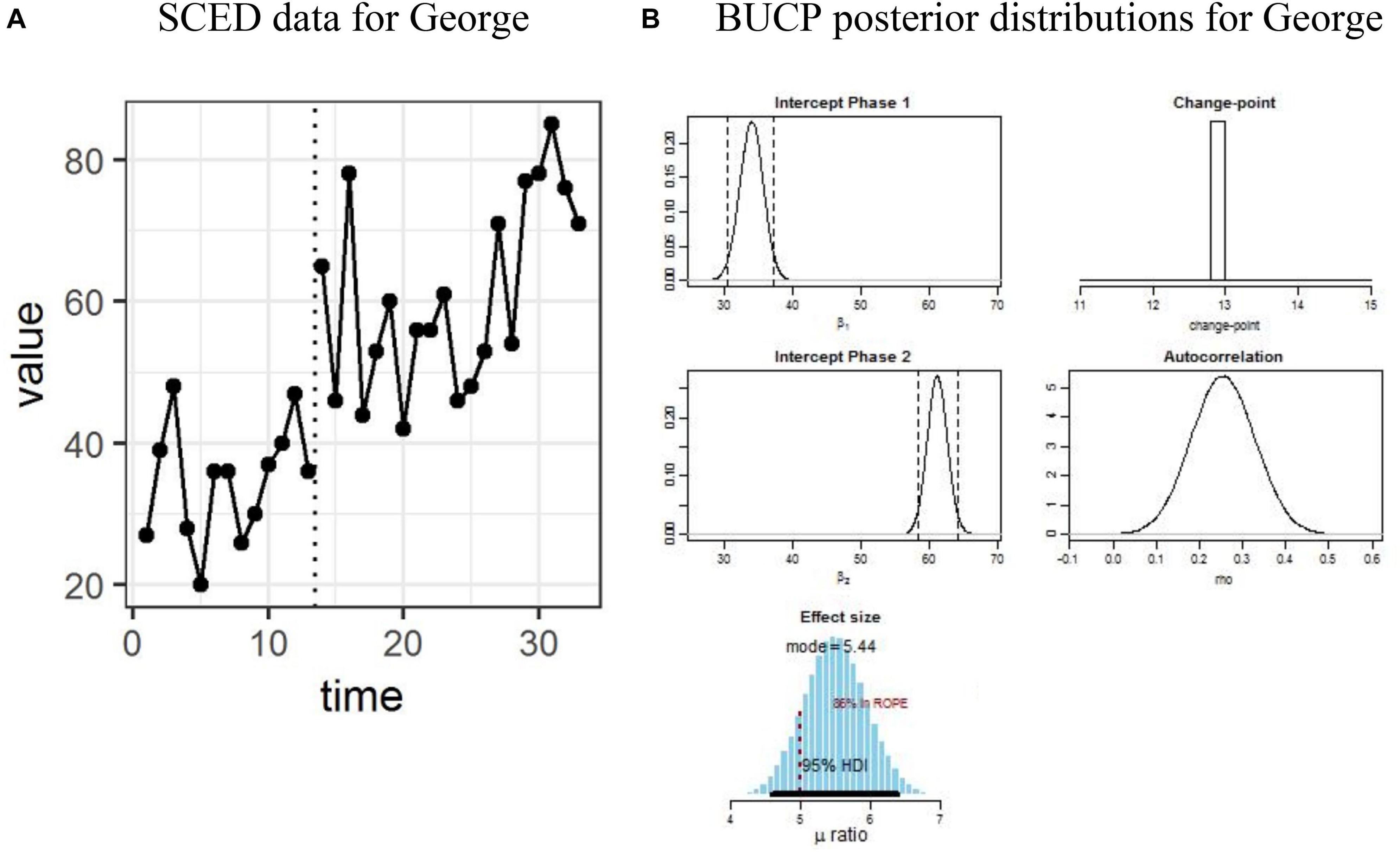
-
Prior (before time=13): Looking at the baseline data (left of the dotted line), your belief is that George's score fluctuates around a mean of about 35-40. Your prior for the effect of the intervention is that it might cause a change, but you're unsure of the magnitude or direction.
-
Likelihood (after time=13): You observe the data points from time 13 onwards. There is a clear, immediate jump in the scores.
-
Posterior (Panel B): A formal Bayesian analysis produces these posterior distributions, which represent your updated beliefs.
- Change-point: This plot shows the probability that the change occurred at any given time point. It's overwhelmingly confident the change happened exactly at time 13, matching the intervention. Your belief that the intervention caused the change is now very strong.
- Intercepts: These show your updated beliefs about the average score before (Phase 1) and after (Phase 2) the intervention.
- Effect size: This is the posterior distribution for the magnitude of the intervention's effect. The mode is at 5.44, and the 95% Highest Density Interval (analogous to a confidence interval) is entirely positive. Your belief is now that the intervention has a strong positive effect.
This is the end-product of Bayesian reasoning: not a simple p-value, but a rich, multi-faceted understanding of the change process, complete with quantifiable uncertainty.
Conclusion
Today we've reframed Bayesian statistics from a purely academic tool into a practical, conceptual framework for data-informed coaching. You've seen how it provides a formal language for the iterative process of learning about your client and adapting your strategies based on evidence.
Key Takeaways:
- Bayesian reasoning is a model for learning under uncertainty. It moves beyond "yes/no" answers to "how confident am I?"
- The core workflow is a cycle: formulate a Prior belief, update it with data (the Likelihood), and arrive at an updated Posterior belief.
- Sequential updating allows you to refine your assessment of an intervention's effectiveness in real-time as new client data comes in.
- This approach aligns perfectly with the adaptive, N-of-1 nature of coaching, providing a structured and defensible method for making decisions about client care.
In our previous lessons, we designed the experiment and the data collection tools. Today, we've explored a sophisticated philosophy for interpreting the results. In our next lesson, we will complement this by looking at more traditional frequentist statistical tests (e.g., paired t-tests). These can provide simpler pre-post analyses and, when paired with the data visualization techniques we will also cover, give you a flexible toolkit for both your own analysis and for communicating progress to your clients.