Hello! Welcome to the final lesson in our module on building dynamic MIS reports.
In our last session, we created summary tables for trend analysis, enabling us to see how incident counts change month-over-month and week-over-week. Your Summary sheet is now populated with powerful metrics and PivotTables. But before we present these numbers to any stakeholder, we must ask a critical question: "Are they correct?"
This lesson is dedicated to answering that question. We will focus on the learning outcome: Perform data reconciliation to validate that summary report figures match the source data totals.
Data reconciliation is the process of ensuring that the numbers in your summary reports perfectly match the raw data. Your background in handling sensitive legal and cybersecurity data has surely emphasized the importance of precision and accuracy. In MIS, this process is our quality assurance—it's what makes our reports credible and trustworthy.
We'll cover three levels of reconciliation:
- A quick "grand total" check.
- Building a "live" validation section using formulas.
- A powerful PivotTable technique for comparing two different datasets.
Let's open your incident tracker file and make sure your reports are bulletproof.
Part 1: The "Grand Total" Check
The simplest and quickest form of reconciliation is to compare the grand totals in your summary against the totals from your source data. This is your first line of defense against major errors.
Let's try this with the KPIs you built in a previous lesson on your Summary sheet.
- Navigate to your Summary sheet. Find the KPI for "Total Incidents" that you created using
COUNTAor a similar function. Note the number. - Now, go to your Tracker sheet. Click on the header of the
Incident IDcolumn in your Excel Table to select all the incident IDs. - Look at the Status Bar at the bottom of your Excel window. You should see a
Countthat tells you the total number of non-blank cells. - Do these two numbers match? They should.
Now let's check a conditional total:
- On the Summary sheet, find your KPI for "Open Incidents", which you calculated with
COUNTIFS. Note the number. - Go back to the Tracker sheet. Click the filter dropdown arrow on the
Statuscolumn header and filter for "Open" status only. - Select the
Incident IDcolumn again. - Check the
Countin the Status Bar. Does it match your KPI?
This manual check is excellent for a quick validation, but it's not dynamic. If you change your data, you have to remember to perform the check again. Let's build something more robust.
Part 2: Formula-Based Reconciliation Checks
A more reliable method is to build a small, dedicated "Reconciliation" or "Validation" section right on your Summary sheet. This section will contain formulas that automatically check your KPIs against the source data.
Let's create a validation check for your main KPIs. On your Summary sheet, find some empty space and set it up like this:
| Metric | Summary Figure | Source Figure | Difference |
|---|---|---|---|
| Total Incidents | |||
| Open Incidents | |||
| Closed Incidents |
Now, let's fill it in:
- Summary Figure column: In this column, simply link to the cells that contain your existing KPI calculations. For "Total Incidents", the formula might just be
=B2(if your KPI is in cell B2). - Source Figure column: In this column, you will write new formulas that calculate the figures directly from the
Trackersheet.- For "Total Incidents":
=COUNTA(Incident_Tracker[Incident ID])(assuming your table is namedIncident_Tracker). - For "Open Incidents":
=COUNTIF(Incident_Tracker[Status], "Open") - For "Closed Incidents":
=COUNTIF(Incident_Tracker[Status], "Closed")
- For "Total Incidents":
- Difference column: In this column, subtract the Source Figure from the Summary Figure. For the first row, the formula would be
=B10-C10(adjust cell references as needed).
If your report is accurate, the "Difference" column should show 0 for all metrics. This section now acts as a "health check" for your report. If a zero ever changes, you know there's a discrepancy that needs immediate investigation.
The article below discusses this best practice of building in validation checks to ensure data accuracy.
How to Build a Financial Report in Excel?
This article on building financial reports emphasizes the importance of data accuracy. Please read the short section on this topic.
In the article, find the section titled 'Best Practices for Building Reports in Excel' and read the sub-section '1. Ensuring data accuracy'. This reinforces the concept of creating reconciliation formulas to compare totals and identify discrepancies.
This method is great for validating summary figures against a single source table. But what if you need to compare two separate lists?
Part 3: The PivotTable Method for Comparing Two Datasets
This is an incredibly powerful technique used by analysts everywhere. Imagine you receive a list of incidents from another department and you need to compare it to your own tracker to find what's missing or what's different. This is a common task for an MIS Executive.
The core idea is to:
- Combine both lists into one large table.
- Add a "Source" column to label which list each row came from.
- Use a PivotTable to count occurrences of each item by source.
Let's simulate this.
Create a Second Dataset
- On your
Trackersheet, select about 20 rows of your data and copy them. - Create a new worksheet and name it
Team_B_List. Paste the data there. - Now, introduce some discrepancies to simulate a real-world scenario:
- Delete 2-3 rows entirely from the
Team_B_List. - On one row, change the
Severityfrom "High" to "Medium". - On another row, change the
Incident IDto something new (e.g., changeINC-005toINC-999).
- Delete 2-3 rows entirely from the
You now have two similar, but not identical, lists. Let's reconcile them.
Execute the Reconciliation
The following video provides a perfect walkthrough of the method. While it uses a bank reconciliation as an example, the steps are universal. We will adapt it for our incident lists.
Compare 2 Excel Sheets (Easy Bank Reconciliation)
This video from Excel Campus demonstrates the definitive method for reconciling two lists using a PivotTable. Follow along with the steps using your Tracker data and the Team_B_List you just created.
Watch from 00:22 to 10:38. As you watch, perform these steps in your own file: Combine Data (00:22): Create a new sheet named Recon_Data. Copy all data from your Tracker sheet and paste it here. Then, copy all data from Team_B_List and paste it directly underneath the first set of data in Recon_Data. Add the 'Source' Column (01:25): Add a new column called 'Source'. For all the rows from your original tracker, fill this column with the text "MyTracker". For the rows from Team B's list, fill it with "TeamB". Convert to Table: Select all the data in Recon_Data and press Ctrl+T to format it as an Excel Table. Create & Analyze with a PivotTable (04:20): Create a PivotTable from your new Recon_Data table. Configure it as follows: Rows: Drag Incident ID here. Columns: Drag Source here. Values: Drag Incident ID here (it will become Count of Incident ID). Drill Down (08:30): The video shows how to add more fields like 'Date' or 'Description' to the Rows area to investigate discrepancies further. Try adding the Severity field to the Rows area below Incident ID to see the impact of the change you made.
After building the PivotTable, you can instantly see the discrepancies:
- Items with a
1under MyTracker and a1under TeamB are matched. - Items with a
1under one source but a blank under the other are present in one list but missing from the other. - By filtering the PivotTable to show only the mismatches, you can quickly generate a list of items to investigate.
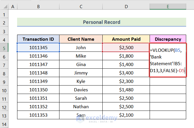
Here is a static image using a VLOOKUP to achieve a similar row-by-row comparison, another valid reconciliation technique for when your data is structured side-by-side.
Conclusion
Excellent work. You have just learned one of the most important quality control processes in MIS reporting. Building a report is one thing; proving it is correct is another, and it is a skill that builds immense trust with your stakeholders.
Key Takeaways:
- Reconciliation is Essential: It's a non-negotiable step to ensure the accuracy and credibility of your reports.
- Start Simple: Always perform a quick "Grand Total" check as a first pass.
- Automate with Formulas: Create a dedicated validation section in your reports that uses formulas to provide a "live" check of your KPIs against source data.
- Master the PivotTable Method: For comparing two separate datasets, combining them with a "Source" column and using a PivotTable is the most efficient and powerful technique.
You have now completed the module on building dynamic MIS reports. You have learned to structure data, write formulas, analyze trends, and now, validate your work.
In our next lesson, we will begin the exciting process of bringing all this work together. We will start Module 9: Creating Interactive Dashboards by planning a one-page dashboard layout to display your KPIs and charts in a professional, user-friendly format.