Hello! Welcome to the final lesson in our module on lookup formulas.
In our previous lessons, you mastered retrieving data using VLOOKUP, XLOOKUP, and the powerful INDEX/MATCH combination. However, you've probably noticed that if a lookup value isn't found, Excel returns an #N/A error. In a professional MIS report, these errors are not just visually jarring; they can also break downstream calculations like sums or averages.
Today, we'll tackle this head-on. Our goal is to wrap lookup formulas with IFERROR to handle and display clean results instead of #N/A errors. This simple but vital function will elevate your reports from functional to professional, a key skill for any MIS Executive.
1. Understanding the Problem and the Solution: The IFERROR Function
Before we apply IFERROR to lookups, let's understand why it's so important. An error in one cell can create a chain reaction, causing other formulas that depend on it to fail as well. This can compromise your entire report.
The IFERROR function is Excel's elegant solution to this problem. It works like this:
- It evaluates a formula or value you give it.
- If the formula calculates correctly,
IFERRORreturns that result. - If the formula results in any type of error (
#N/A,#DIV/0!,#REF!, etc.), it returns a custom value that you specify instead.
The syntax is straightforward:=IFERROR(value, value_if_error)
value: The formula or cell you want to check for errors (e.g., yourVLOOKUPformula).value_if_error: What to show if an error is found. This can be text (like "Not Found"), a number (like 0), or even an empty string ("") to display a blank cell.
To see why this is so critical in MIS reporting, let's watch a short video. While this example uses a #DIV/0! error, the principle is exactly the same for the #N/A errors we get from lookups.
The Excel IFERROR Function: Clean up Your Excel Errors
This video from Technology for Teachers and Students clearly demonstrates how a single error can disrupt other calculations, like an AVERAGE formula, and how IFERROR elegantly solves the problem.
Watch from 01:24 to 03:32. Pay attention to two key things: How the #DIV/0! errors cause the AVERAGE formula to also return an error. How wrapping the initial calculation in IFERROR to return a 0 instead of an error fixes the AVERAGE formula automatically.
2. Applying IFERROR to Your Lookup Formulas
Now let's apply this directly to the lookup functions you've learned. The process is the same for all of them: you simply "wrap" your existing lookup formula inside IFERROR.
=IFERROR( YourVlookupOrIndexMatchFormula , "YourCustomOutput" )
Handling Errors with VLOOKUP
Let's start with VLOOKUP. This is the most common combination you'll encounter in existing spreadsheets.
IFERROR with VLOOKUP Excel: Say Goodbye to Errors in Minutes
This quick tutorial from Productivity Land gets straight to the point, showing you exactly how to combine IFERROR and VLOOKUP.
Watch from the beginning to 01:59. Notice how the #N/A errors are instantly replaced with a more user-friendly message.
As you saw, you can replace the error with any text you want. For a more detailed guide with different output options, the following article is an excellent reference.
Excel IFERROR & VLOOKUP - trap #N/A and other errors
The article 'Excel IFERROR & VLOOKUP' on Ablebits.com provides clear, practical examples of different ways to handle errors.
Read the section 'IFERROR VLOOKUP formula to handle #N/A and other errors', including both Example 1 and Example 2. This will show you how to replace errors with: Custom text (e.g., "Not found") A blank cell ("") The number zero (0)
Handling Errors with INDEX/MATCH
The principle is identical for the INDEX/MATCH combination you learned in the last lesson. You wrap the entire INDEX(...) formula with IFERROR.
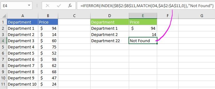
By wrapping your complex INDEX/MATCH formula, you ensure that if either the row or column lookup fails, you still get a clean, predictable output.
3. Hands-On Practice & A Word of Caution
Let's apply this to the incident tracking scenario from our previous lesson.
Scenario:
You have your INDEX/MATCH formula from the last lesson that finds the number of incidents for a given type and quarter.
| Incident Type | Q1 | Q2 | Q3 | Q4 |
|---|---|---|---|---|
| Phishing | 150 | 185 | 160 | 210 |
| Malware | 45 | 30 | 55 | 40 |
| Data Leak | 12 | 15 | 8 | 18 |
| Ransomware | 5 | 2 | 7 | 4 |
Let's say a user enters an invalid incident type, like "Virus", in your lookup cell. Your INDEX/MATCH formula would currently return #N/A.
Your Task:
Modify your INDEX/MATCH formula to handle this error. If an incident type or quarter is not found, the formula should display 0 instead of an error.
Click here to see the solution formula
Assuming your previous formula was:=INDEX($B$2:$E$5, MATCH(G2, $A$2:$A$5, 0), MATCH(H2, $B$1:$E$1, 0))
The new, improved formula would be:=IFERROR(INDEX($B$2:$E$5, MATCH(G2, $A$2:$A$5, 0), MATCH(H2, $B$1:$E$1, 0)), 0)
Now, if G2 contains "Virus", or H2 contains "Q5", the formula will return 0, which can be safely used in further calculations.
A Word of Caution
IFERROR is powerful, but it's important to know that it catches all types of errors. This is usually what you want, but it can occasionally hide other problems. For example, if you accidentally mistype a range name in your VLOOKUP formula, it will generate a #NAME? error. IFERROR will catch this and display "Not Found", which might lead you to believe the lookup value is missing when the formula itself is broken.
For professional work, always double-check your formulas before wrapping them in IFERROR.
4. Advanced Application: Sequential Lookups
One of the most powerful uses of IFERROR in an MIS role is to chain lookups together. Imagine you need to find an employee's details, but they could be in one of three different spreadsheets (e.g., 'Sales_Team', 'Ops_Team', 'HR_Team').
You can nest IFERROR functions to create a sequence:
- Try to find the employee in 'Sales_Team'.
- If that returns an error, try to find them in 'Ops_Team'.
- If that also returns an error, try to find them in 'HR_Team'.
- If none are successful, then return "Employee Not Found".
This is a very practical and robust technique for consolidating data from different sources.
Excel IFERROR & VLOOKUP - trap #N/A and other errors
The Ablebits.com article we looked at earlier has an excellent section on this advanced technique. This is a great example of how you can solve complex, real-world data problems with a clever combination of simple functions.
Read the final section of the article, 'How to do sequential VLOOKUPs in Excel'. Focus on understanding the logic of how the nested IFERROR functions pass control from one VLOOKUP to the next if an error occurs.
Key Takeaways
- Unmanaged errors like
#N/Alook unprofessional and can break other formulas in your report. - The
IFERRORfunction is the standard solution for handling errors gracefully. Its syntax is=IFERROR(value, value_if_error). - You can wrap
VLOOKUP,INDEX/MATCH, or any other formula insideIFERRORto control what's displayed when an error occurs. - You can return custom text, a number (like 0), or a blank cell (
"") to keep your reports clean and functional. - Nesting
IFERRORfunctions allows you to perform powerful sequential lookups across multiple sheets or tables.
Next Lesson
Congratulations on completing the module on lookup formulas! You can now confidently retrieve data from tables and manage any errors that arise.
In our next module, "Data Cleaning and Validation Techniques," we will shift our focus from retrieving data to preparing it. We'll start by learning how to use text functions (TRIM, CLEAN, UPPER, PROPER) to standardize text data, a fundamental first step in ensuring your analysis is accurate.