Hello! Welcome to the final lesson in our module on creating interactive dashboards.
In our last session, we added another layer of interactivity by incorporating dropdown lists using Data Validation. You learned how to create dynamic lists that update automatically, providing a space-efficient way for users to filter report data.
So far, we have built a fully functional dashboard. It has dynamic charts, interactive slicers, and dropdowns. Now, it's time for the final, crucial step: making it look professional.
Today's lesson is all about design. Our goal is to apply consistent formatting, alignment, and design principles to create a presentation-ready dashboard. An analyst who can present data clearly and professionally stands out. A well-designed report is not just about aesthetics; it's about making your data more understandable, persuasive, and credible to your audience, whether they are team leads or senior management.
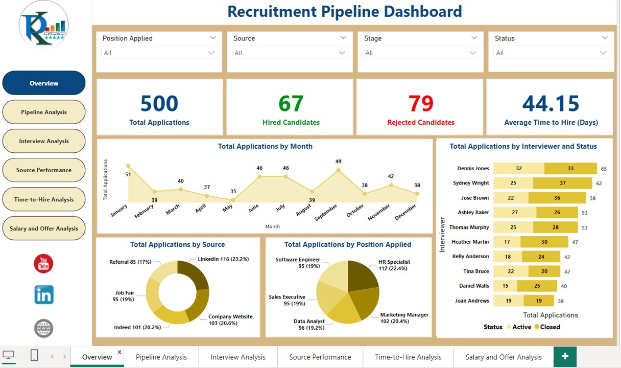
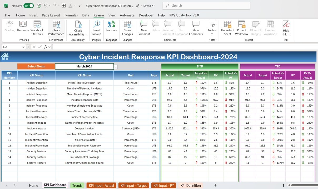
Let's look at a couple of examples of what we're aiming for. Notice the clean layout, consistent colors, and clear titles. These are the kinds of professional reports you'll be able to build.
1. Planning Your Layout: The Power of Wireframing
Before you start formatting individual elements, it's essential to have a plan. The best practice is to create a simple "wireframe"—a rough sketch of your dashboard's layout. This helps you decide where to place your most important information (KPIs), your charts, and your filters before you get lost in the details of colors and fonts.
Create interactive excel dashboard in 5 simple steps #exceldashboard #exceltutorial #pivottable
This short video from Skillnator introduces the concept of wireframing. Watch how a simple sketch provides a blueprint for the entire dashboard, saving a lot of time later.
Watch the section on wireframing (01:51 - 04:11). You don't need special software; a simple layout using shapes in Excel or even a pen and paper is enough. The key is to think about the structure first.
2. Creating a Clean and Consistent Canvas
A professional dashboard doesn't look like a standard Excel grid. The first step is to create a clean "canvas" that focuses the viewer's attention on your data.
Key Steps for a Clean Canvas:
- Set a Background Color: Use a neutral, non-distracting color for your dashboard's background. Often a light grey or a muted brand color works well. This immediately separates it from a regular worksheet.
- Hide Gridlines: Go to the
Viewtab and uncheckGridlines. This removes the default cell grid, creating a cleaner look. - Hide Unused Rows and Columns: This is a simple but powerful trick. It prevents users from scrolling away from your dashboard and makes it feel like a contained application.
4 Hidden Excel Dashboard Design Tips for Beautiful Reports
This article from XelPlus explains how to hide unused rows and columns to give your dashboard a polished, focused feel.
Read Tip #2: Hide Unused Rows and Columns. The instructions show you how to quickly select and hide all columns to the right of your dashboard and all rows below it.
Establishing a Color Theme
Consistency is the most important rule in dashboard design. Instead of picking colors at random, establish a consistent palette.
- Page Layout Themes: The easiest way is to use Excel's built-in themes. Go to
Page Layout>Colorsand select a theme. All your charts and tables will update to this new palette. - Custom Color Palette: For a more branded look, you can create a custom color palette that all your dashboard elements will inherit.
Create interactive excel dashboard in 5 simple steps #exceldashboard #exceltutorial #pivottable
The Skillnator video we saw earlier has an excellent demonstration of setting up a custom color theme. This ensures every new chart or pivot table you create will automatically use your chosen brand colors.
Watch the section on setting up a custom color palette (23:07 - 24:36). Pay attention to how changing 'Accent 1' in the 'Customize Colors' dialog immediately influences the look of all objects on the sheet.
3. Formatting Key Dashboard Elements
With a clean canvas and a color theme, you can now format the individual components of your dashboard.
Interactive Excel Dashboard Tutorial in 3 Steps (+ FREE Template)
This comprehensive video from MyOnlineTrainingHub is a masterclass in dashboard formatting. We will watch it in segments to learn how to format each part of a dashboard, from KPI cards to charts and tables.
Please watch the following sections. You'll see an entire dashboard built from a design perspective. Dashboard Canvas and KPI Cards (00:44 - 03:44): See how to set the background color and create professional-looking KPI cards using shapes and icons. This is how you display your main numbers prominently. Formatting a PivotTable (07:48 - 10:15): Learn how to apply your color theme to a pivot table, rename headers for clarity, and use conditional formatting (Data Bars) to make the table more visual. Formatting Charts (10:33 - 15:37): This is a critical section. Observe how to: Hide unnecessary field buttons. Remove gridlines and borders. Apply consistent colors. Use data labels effectively. Add a trendline for context. Final Polishes (15:37 - 17:59): See how to add subtle shadows for depth and use shapes to create clean titles for your tables.
Upgrading Your Slicers
Default slicers are functional, but they can look clunky. With a bit of customization, you can make them look like sleek, clickable buttons that integrate perfectly with your design.
Create interactive excel dashboard in 5 simple steps #exceldashboard #exceltutorial #pivottable
Let's return to the Skillnator video for one last, brilliant tip on formatting slicers. This will take your dashboard's user interface to the next level.
Watch the segment on formatting slicers (31:22 - 33:24). The key takeaways are changing the number of columns to arrange the buttons horizontally, and creating a custom slicer style to remove the border and header.
4. Alignment and Organization
A well-aligned dashboard looks organized and intentional. Excel's Align tools are your best friend here.
- To align multiple objects (charts, shapes, slicers):
- Hold down the
Ctrlkey and click on each object to select them all. - Go to the
Shape FormatorPicture Formattab that appears. - Click
Alignand choose an option likeAlign Top,Align Middle, orDistribute Horizontally.
- Hold down the
For complex dashboards with many overlapping objects, the Selection Pane is an invaluable tool for managing everything.
4 Hidden Excel Dashboard Design Tips for Beautiful Reports
The XelPlus article we viewed earlier also has a great tip on using the Selection Pane. It's like a table of contents for all the objects on your sheet.
Read Tip #3: Select Objects From the Selection Pane. You'll see how you can use it to select, hide, and rename objects, which is extremely helpful when your dashboard gets crowded.
5. Your Turn: The Dashboard Makeover
Now, let's apply these design principles to your Incident_Tracker.xlsx file. Open the file and go to your Dashboard sheet. We're going to give it a complete professional makeover.
-
Prepare the Canvas:
- Select the entire
Dashboardsheet and give it a light grey fill color. - Go to the
Viewtab and uncheckGridlines. - Identify the rightmost column of your dashboard content. Select the column to its right, press
Ctrl+Shift+Right Arrowto select all remaining columns, then right-click andHide. - Do the same for the rows below your dashboard content (
Ctrl+Shift+Down Arrowto select, thenHide).
- Select the entire
-
Set a Color Theme:
- Go to
Page Layout>Colors. Choose a theme you like (e.g., 'Aspect' used in the video, or 'Blue Warm'). Notice how your chart colors update automatically.
- Go to
-
Layout and Alignment:
- Arrange your charts, slicers, and dropdown list into a logical layout. A common pattern is KPIs and filters at the top, with detailed charts below.
- Select your charts and use
Shape Format>Align>Align Topto make sure they are perfectly level. UseDistribute Horizontallyto space them out evenly.
-
Format the Elements:
- Charts: For each chart, right-click the grey field buttons (like "Sum of...") and select
Hide all field buttons on chart. Remove borders and add titles. - Slicers: Select your slicer. In the
Slicertab, change theColumnsto match the number of items (e.g., if you have 3 priorities, set it to 3 columns). Follow the video's steps to create a new slicer style with no border and no header. - Title: Instead of typing the title in a cell, go to
Insert>Shapes, choose a rectangle, and draw it across the top of your dashboard. Format it with a darker color from your theme, and type a title like "Incident Management Dashboard". Make the font bold and white.
- Charts: For each chart, right-click the grey field buttons (like "Sum of...") and select
-
Review and Refine:
- Take a step back and look at your dashboard. Is it easy to understand? Is anything distracting? Make small adjustments to spacing and alignment until it looks clean and professional.
Conclusion
Congratulations! You've moved beyond just making things work and are now learning how to make them presentable and impactful. This is a critical skill for an MIS Executive, as the reports you build are your primary way of communicating insights to the business.
Key Takeaways:
- Plan First: Wireframe your layout before you begin formatting.
- Create a Clean Canvas: Use a solid background and hide gridlines and unused cells.
- Be Consistent: Use a deliberate color theme and consistent fonts. This is the single most important design rule.
- Remove Clutter: Hide unnecessary chart buttons, borders, and legends to let the data speak for itself.
- Align Everything: Use the alignment tools to create a structured, organized look.
- Format Intentionally: Customize slicers, charts, and tables to look polished and professional.
In our next module, we will significantly expand your data handling capabilities. We'll dive into Power Query, a powerful tool for automating the process of importing and cleaning data from multiple sources. Our first lesson will focus on a very common MIS task: combining data from all Excel files within a single folder.