Create a Dropdown List with Data Validation

1. What is a Data Validation List?

At its core, Data Validation is an Excel feature designed to control what data is entered into a cell, ensuring accuracy and consistency. One of its most common uses is to create a dropdown list that restricts a user's choice to a predefined set of options.

For an MIS dashboard, this is incredibly useful. Instead of letting a user type a department name (and risk a typo like "Finanace" instead of "Finance"), you can provide a dropdown list of approved department names. This guarantees the input is always correct, which is critical for the formulas that will use this selection.

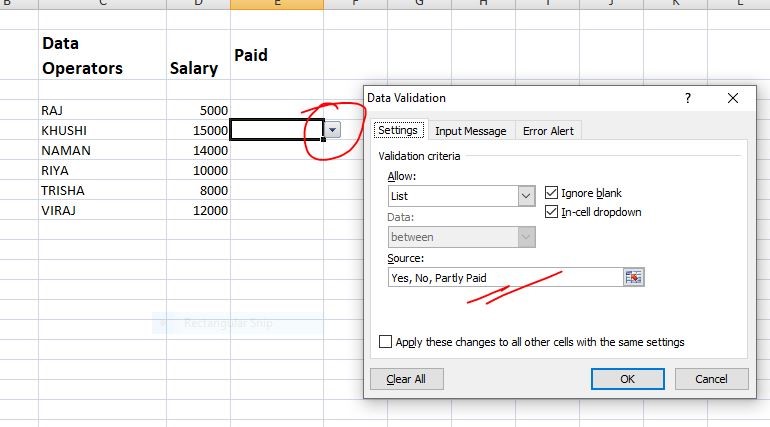
To start, let's get familiar with the basic methods of creating a dropdown list.

2. Building Dynamic and Professional Dropdown Lists

For an MIS professional, static lists are often not enough. Your source data changes—new employees are added, products are launched, or statuses are updated. You need your dropdown lists to update automatically without you having to manually redefine the source range every time. This is where dynamic lists come in.

Method 1: The Table + Named Range Technique

This is a robust and widely-used method. The process is:

1. Put your source list items in a range of cells.
2. Convert that range into a structured Excel Table (Insert > Table or Ctrl+T).
3. Define a Named Range that refers to the data column in that table.
4. Use the Named Range as the source for your Data Validation list.

Because Excel Tables automatically expand to include new data, and the Named Range refers to the table column, your dropdown list will magically update whenever you add or remove items from the table.

This next clip from the same video demonstrates this powerful technique perfectly.

Method 2: Creating a Unique List from a Data Column

This is another extremely common scenario in MIS work. Imagine you want a dropdown list of every employee who has an incident assigned to them. The 'Assigned To' column in your main data table will have many duplicate names. You need a list of unique names for your dropdown.

For this, we can use one of two methods, as explained in the following article.

3. Your Turn: Add a Dropdown Selector to Your Dashboard

Let's apply these professional techniques to your Incident_Tracker.xlsx file. We will add a dropdown list on the dashboard to let a user select a specific person and see their stats.

1. Open Incident_Tracker.xlsx.

2. Create a 'Lists' Worksheet: It's best practice to keep the source for your dropdowns organized. Create a new worksheet and name it Lists.

3. Generate a Unique, Sorted List:

   • In cell A1 of your new Lists sheet, add a header, e.g., "AssignedToList".
   • In cell A2, type the following formula to get a unique, sorted list of names from your main data table:

     =SORT(UNIQUE(Incident_Table[Assigned To]))
     

   • Excel will automatically "spill" a list of unique names into the cells below A2.

4. Create a Dynamic Named Range:

   • Select cell A2 on the Lists sheet.
   • Go to the Formulas tab > Define Name.
   • Name: AssignedToList
   • Refers to: Enter =Lists!$A$2#
   • The # symbol at the end is crucial. It tells Excel to refer to the entire dynamic spill range, so the named range will automatically adjust if new names are added to the list.
   • Click OK.

5. Create the Dropdown on the Dashboard:

   • Go to your Dashboard sheet. Select a cell where you want the dropdown to appear (e.g., cell D3).
   • Go to the Data tab > Data Validation.
   • In the Data Validation dialog box:
     • Allow: List
     • Source: =AssignedToList
     • Make sure 'In-cell dropdown' is checked.
   • Click OK.

You now have a dynamic dropdown list in cell D3 of your dashboard! When you add a new incident with a new person's name in your Tracker sheet, their name will automatically appear in this dropdown list after you refresh your data.

How is this used?

Unlike a slicer, a dropdown list doesn't automatically filter anything. It simply places a value in a cell. You make it interactive by linking your dashboard formulas to this cell.

For example, on your Calculations sheet, you could create a new set of summary stats that reference your dropdown cell. A formula might look like this:
=COUNTIFS(Incident_Table[Assigned To], Dashboard!$D$3, Incident_Table[Status], "Open")

This formula counts open incidents only for the person selected in the dropdown on the dashboard. You would then link your dashboard charts or KPI cards to these new summary cells.

Conclusion

You've now learned a second powerful method for adding interactivity to your dashboards. Dropdown lists are a fundamental skill for any MIS role, as they ensure data integrity while providing a clean user interface.

Key Takeaways:

• Data Validation is used to create dropdown lists, which control user input.
• For professional use, always source your lists from a cell range, ideally on a separate Lists or Settings sheet.
• To create dynamic lists that update automatically, use the Table + Named Range method or the SORT(UNIQUE()) function with a dynamic array named range (#).
• A dropdown cell is an input cell. You make it interactive by referencing it in your summary formulas (SUMIFS, COUNTIFS, etc.).

In our next and final lesson for this module, we will shift our focus from functionality to presentation. We'll learn how to apply consistent formatting, alignment, and design principles to transform your functional dashboard into a polished, presentation-ready report.