Hello! Let's continue building your data visualization skills.
In the previous lesson, you learned how to create and format the three most essential chart types: bar, column, and line charts. You now know how to represent comparisons and trends visually, which is a core skill for any MIS role.
Today, we'll tackle a common challenge in reporting: how to show two different types of data on the same chart. Imagine you want to display monthly sales revenue (in thousands of dollars) alongside the profit margin (as a percentage). Plotting these on the same axis would make the small percentage values almost invisible next to the large dollar amounts.
This lesson focuses on solving that problem by teaching you how to build a combination chart to visualize two different metrics together. This technique is invaluable for creating rich, insightful reports that show the relationship between different KPIs.
The Problem with Different Scales
When two data series have vastly different scales, putting them on the same chart can be misleading or unreadable. A secondary axis allows you to plot one data series against a separate scale on the right-hand side of the chart.
To see why this is so important, let's watch a quick video that perfectly illustrates the problem and introduces the solution.
Add Secondary Axis in Excel Charts (in a few clicks)
This clip from the TrumpExcel channel clearly demonstrates what happens when you try to chart data with different scales on a single axis.
Watch the first 55 seconds of the video (0:09 - 0:55). Notice how the 'Profit Margin' bars are barely visible compared to the 'Sales' bars, making the chart ineffective.
As you can see, without a way to handle the different scales, one part of your data story is completely lost. The combination chart with a secondary axis is the solution.
Creating a Combination Chart
A combination chart, or combo chart, uses two or more chart types (like columns and a line) in one. To make it work with different data scales, you assign one of the data series to a secondary axis.
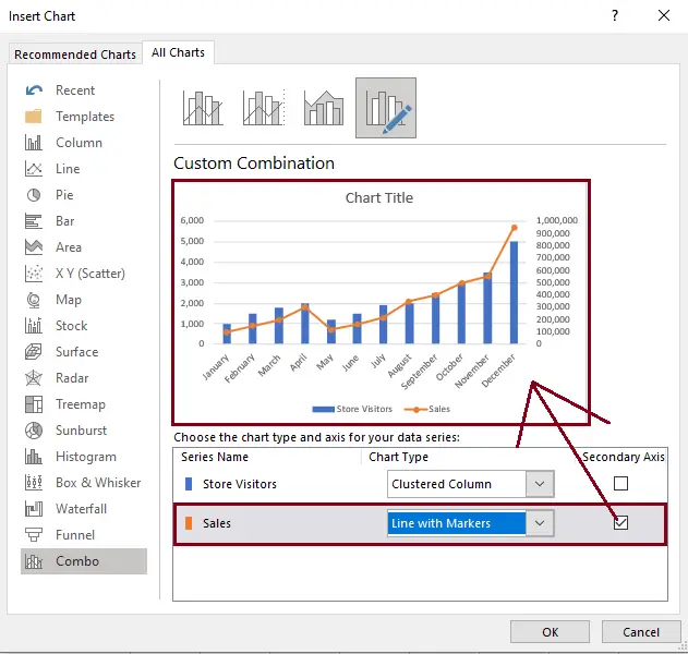
Let's walk through the creation process. There are a few ways to do this, but the most straightforward is to use the "Combo" chart option from the Insert Chart dialog.
This image shows the exact dialog box where you'll configure your chart. You can choose the chart type for each data series and check a box to move a series to the secondary axis.
Now, let's watch a detailed video tutorial that covers the end-to-end process.
How to Create a Combination Chart (Combo Chart) in Excel
The Data Design Style channel provides a great tutorial on creating combo charts. It covers both a simple and a more complex example.
Watch from the beginning to 05:09. Pay close attention to these two methods: Direct Creation (0:00 - 02:14): The video first shows how to use the Insert > Recommended Charts > All Charts > Combo menu. This is the quickest way for simple datasets. Starting with a Column Chart (02:14 - 05:09): For more complex data, the video recommends a powerful technique: start with a standard column chart, clean up the data selection, and then right-click a series to change its chart type. This gives you more control and is a best practice for professional work.
Your Turn: Track Sales and Growth
Let's apply this with a hands-on exercise. Imagine you're an MIS Analyst preparing a report on monthly product sales and growth.
Data:
Create a new Excel sheet and enter the following data:
| Month | Revenue ($) | Units Sold |
|---|---|---|
| Jan | 150,000 | 7,500 |
| Feb | 165,000 | 8,100 |
| Mar | 182,000 | 8,500 |
| Apr | 175,000 | 8,200 |
| May | 198,000 | 9,300 |
| Jun | 210,000 | 9,900 |
Task:
Create a combination chart that visualizes Revenue and Units Sold over time.
- Select your data range (including the headers).
- Go to the
Inserttab, click theCombochart icon, and selectCreate Custom Combo Chart. - In the dialog box, configure your chart as follows:
- For the
Revenue ($)series, set the chart type toClustered Column. It will use the primary axis by default. - For the
Units Soldseries, set the chart type toLine with Markers. - For this same
Units Soldseries, check theSecondary Axisbox.
- For the
- Click
OK.
You should now have a chart that shows revenue as columns measured on the left axis and the number of units sold as a line measured on the right axis.
Formatting for a Professional Report
A default combo chart needs formatting to be clear and professional. You must label both axes and ensure the colors and legend are easy to understand.

Let's learn some key formatting techniques specifically for combo charts.
How to Create a Combination Chart (Combo Chart) in Excel
Let's return to the Data Design Style video to learn some excellent formatting tips that will make your charts presentation-ready.
Watch from 05:09 to 06:45. Focus on how the presenter uses formatting to improve clarity: Axis Position: Notice the thought process behind which series belongs on which axis. Color-Coding: A powerful tip is to color the axis title and legend entry to match the data series itself. This makes the chart instantly readable.
Now, apply these formatting principles to the chart you just created:
- Add a Chart Title: "Monthly Revenue and Units Sold".
- Add Primary Axis Title: Click your chart, go to
Chart Design>Add Chart Element>Axis Titles>Primary Vertical. Title it "Revenue ($)". - Add Secondary Axis Title: Go to
Add Chart Element>Axis Titles>Secondary Vertical. Title it "Units Sold". - (Optional) Apply Color-Coding: Try changing the color of the "Units Sold" line and its corresponding axis title to match, as shown in the video.
Conclusion
Excellent work! You have now mastered a data visualization technique that is fundamental to high-quality MIS reporting. Combination charts allow you to tell a more complex and nuanced story by showing the relationship between two different metrics in a single, clear visual.
Key Takeaways:
- Purpose: Use a combination chart to visualize two data series with different scales (e.g., dollars and percentages) or different units (e.g., revenue and quantities).
- Secondary Axis is Key: The secondary axis is what makes the chart work, providing a separate scale for one of the data series.
- Creation Method: The
Insert > Combo > Custom Combo Chartdialog is your main tool for setting up the chart types and assigning the secondary axis. - Formatting is Crucial: Always add titles for both the primary and secondary axes to avoid confusion. Using color to link a data series to its axis is a pro-level technique.
In our next lesson, we will bridge the gap between your data analysis and visualization by learning how to create PivotCharts. These are charts that are directly linked to a PivotTable, allowing you to dynamically filter your visuals and create interactive reports.