Creating Basic Charts from Summary Data

When to Use Which Chart?

Before we start creating charts, it's essential to know which type to choose for your data. The choice depends on the story you want to tell.

• Column or Bar Charts: Use these to compare values across different categories. For example, comparing sales figures for different products, or the number of incidents handled by different team members. A column chart uses vertical bars, while a bar chart uses horizontal bars (often better if you have long category names).
• Line Charts: Use these to show a trend over a continuous period, like days, months, or years. This is perfect for tracking revenue over time, monitoring website traffic, or seeing the number of open support tickets throughout a quarter.

Creating Your First Charts

The fundamental process of creating any chart in Excel is simple: select your data, then choose a chart type from the Insert tab.

Let's watch a detailed walkthrough that covers creating the most common charts from a simple data table. This video is packed with practical tips that will help you work more efficiently.

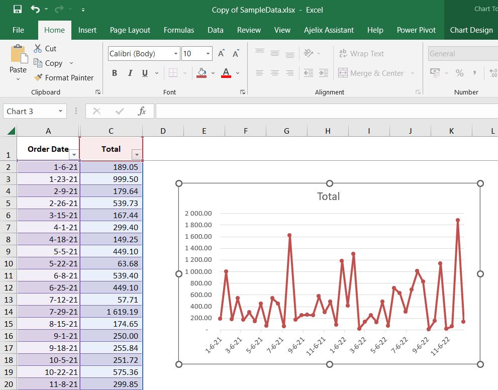
As you saw, creating a basic chart takes only a few clicks.

From Data to Professional Visualization

A default Excel chart is a good start, but for a professional MIS report, you need to refine it. A well-formatted chart is clean, easy to read, and directs the viewer's attention to the key message. This means adding clear titles, labeling your axes, and removing unnecessary clutter.

This next video segment focuses on exactly that—transforming a basic chart into a polished, presentation-ready visual.

A few key formatting principles to always remember:

• Give it a title: The title should clearly state what the chart is showing.
• Label the axes: Ensure the vertical (Y-axis) and horizontal (X-axis) are labeled so the units and categories are clear.
• Add data labels: Sometimes it's helpful to show the exact value of each bar or point.
• Remove clutter: Delete unnecessary elements like gridlines or redundant legends if they don't add value.

Your Turn: Create and Format Charts

Now, let's put this into practice. Please use the sample-data-for-pivot-table.xlsx file.

Scenario: You need to create two visuals for a weekly sales report.

Task 1: Create a Column Chart for Sales by Category

1. First, create a summary of the data. On a new sheet, create a simple PivotTable showing the total Sales for each Category.
2. Select the data in your PivotTable (the categories and their sales totals).
3. Insert a Clustered Column Chart (Insert > Charts > Column).
4. Format the chart:
   • Change the chart title to "Total Sales by Product Category".
   • Add a title to the vertical axis called "Total Sales ($)".
   • Right-click the bars and select "Add Data Labels" to show the sales values on each column.
   • Click on the horizontal gridlines and press Delete to remove them for a cleaner look.

Task 2: Create a Line Chart for Sales Over Time

1. Create another PivotTable. This time, put OrderDate in the Rows area and Sales in the Values area.
2. Group the dates: Right-click on any date in the PivotTable and select Group. In the dialog box, make sure only Months is selected and click OK.
3. Select your new summary data (Months and Sales).
4. Insert a Line with Markers chart (Insert > Charts > Line).
5. Format the chart:
   • Change the chart title to "Monthly Sales Trend".
   • Add an axis title for the vertical axis: "Total Sales ($)".
   • Ensure the chart is easy to read. Adjust colors or line styles if you wish.

Take your time with the formatting. The goal is to produce a chart that you would be confident including in a report for your manager.

Conclusion

Great work today! You've learned how to take summary data and turn it into the three most fundamental chart types used in business: bar, column, and line charts. More importantly, you've learned that creating the chart is just the first step; formatting it for clarity and impact is what truly adds value.

Key Takeaways:

• Choose the right tool: Use column/bar charts for comparing categories and line charts for showing trends over time.
• Start with good data: Your chart is only as good as the summary data it's based on. Always exclude totals from your selection.
• Format for clarity: A professional chart has a clear title, labeled axes, and is free of clutter. Use formatting to tell a story, not to distract.
• Practice shortcuts: Using Alt+F1 will make you much faster at creating reports.

In our next lesson, we will build directly on today's skills. We'll explore how to create combination charts to visualize two different types of data at once (like sales columns and a profit margin line) and how to create PivotCharts, which are charts that are dynamically linked to your PivotTables.