Mastering Chart Formatting for Professional Presentations

The Anatomy of a Chart

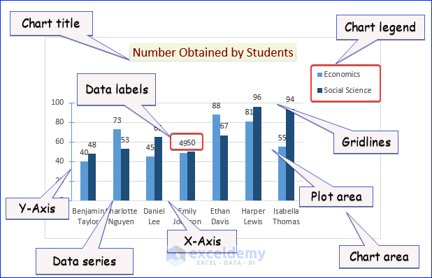
Before we start formatting, let's quickly identify the different parts of a chart we can customize. Each labeled element in the image below can be individually modified.

For this lesson, please open the Excel file from our previous session containing the IncidentData PivotTable and its associated PivotChart. We will be working on that chart directly.

Your Formatting Toolkit in Excel

Excel offers several ways to access formatting options, which gives you a lot of flexibility. The main methods are:

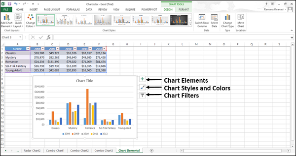
1. The Ribbon: When you select a chart, two contextual tabs appear: Chart Design and Format. These tabs contain a wealth of options for changing the chart's structure and appearance.
2. Chart Shortcut Buttons: Three buttons appear on the top-right of a selected chart. These provide quick access to the most common formatting tasks.
3. Right-Click Menu: Right-clicking on any chart element (like an axis, a bar, or the title) brings up a context-sensitive menu with relevant formatting options.
4. Format Pane: Double-clicking any chart element opens a detailed Format pane on the right side of your screen. This pane gives you the most granular control over every aspect of the selected element.

Hands-On: Polishing Your Incident Status Chart

Let's apply these tools to the PivotChart you created. We'll go element by element to transform it into a professional visual.

1. Crafting a Clear and Dynamic Title

A chart's title should be concise and descriptive. Your current chart likely has a generic title. Let's fix that and add an axis title for clarity.

Now, apply this to your chart:

1. Change the Chart Title: Click on the chart title and change it to "Incident Status by Department".
2. Add a Vertical Axis Title: Click the Chart Elements (+) button, check Axis Titles, and then uncheck Primary Horizontal to keep only the vertical axis title. Change its text to "Number of Incidents".

2. Decluttering for Clarity

Professional charts are clean and easy to read. A common mistake is including too many distracting elements. Let's remove the clutter from your PivotChart.

Your Turn:

1. Hide Field Buttons: Right-click on one of the grey field buttons (e.g., "Status") on your chart and select "Hide All Field Buttons on Chart".
2. Remove the Legend: Click on the legend (which likely shows 'Open' and 'Closed') and press the Delete key.
3. Soften the Gridlines: Click on one of the horizontal gridlines. In the Format pane that appears (or right-click and choose Format Gridlines), change the line color to a light grey. This makes them less distracting but still useful as a guide.

3. Enhancing Data Labels and Bars

With the clutter gone, let's make the core data easier to read by adding data labels and adjusting the bars.

Apply these powerful techniques:

1. Widen the Bars: Click on any of the data bars. In the Format Data Series pane, under Series Options, reduce the Gap Width to around 100%.
2. Add Data Labels: With the bars still selected, click the Chart Elements (+) button and check Data Labels. Position them Inside End for a clean look.
3. Remove the Vertical Axis: Now that you have labels, click on the vertical axis (the one showing the numbers) and press the Delete key. Do the same for the "Number of Incidents" axis title, as it's now redundant.

Your chart should now look much cleaner and more direct.

4. Using Color with Purpose

Color is a powerful tool for communication. Instead of using default colors, let's assign colors that add meaning to the data. For incidents, a common convention is red for "Open" (needs attention) and green for "Closed" (resolved).

1. Click on one of the "Open" bars. This will select all "Open" bars in the chart.
2. Go to the Format tab on the ribbon, click Shape Fill, and choose a shade of red.
3. Now, click on one of the "Closed" bars. This will select all "Closed" bars.
4. Go back to Shape Fill and choose a shade of green.

By using color this way, you're making the chart's story instantly understandable even at a glance.

The Principles of Professional Formatting

You've just applied several key formatting techniques. To ensure you understand the "why" behind these changes, it's helpful to review some established best practices.

The guiding principle is clarity. Every element on your chart should serve a purpose. If it doesn't help the audience understand the data, it's probably just noise.

Conclusion

Well done! You have transformed a default Excel chart into a professional-quality visual. This skill is exactly what hiring managers look for in an MIS role—the ability to not just analyze data, but to present it in a way that is clear, insightful, and ready for decision-makers.

Key Takeaways:

• Declutter Aggressively: Remove redundant legends, busy gridlines, unnecessary axes, and chart field buttons to focus the viewer's attention.
• Be Explicit with Titles and Labels: Use clear chart and axis titles. Use data labels to show precise values, which can often replace an entire axis.
• Use Color Purposefully: Don't just decorate; use color to communicate meaning, such as using red for problems (Open incidents) and green for successes (Closed incidents).
• Format for Readability: Widen bars (adjust Gap Width) and ensure all text is horizontal and easy to read.

In our next lesson, we will begin a new module, "Building Dynamic MIS Reports." We'll shift our focus from visualizing data to designing the source of that data. You'll learn how to design a structured tracker for business processes using an Excel Table, a foundational skill for building any robust MIS system.