Introduction
In our last lesson, you built the dynamic "engine" of our reporting system—the Summary sheet. This calculation layer automatically crunches the numbers from your incident log, giving us live KPIs. Now, it's time to build the "cockpit."
Today, your goal is to construct a one-page interactive dashboard to visualize incident statuses, priorities, and ownership. We will transform the raw numbers from your Summary sheet and the details from your IncidentLog into a clean, professional, and interactive visual report. This is the final and most visible piece of the puzzle, bringing all your hard work together into a tool that allows anyone to understand incident trends at a glance.
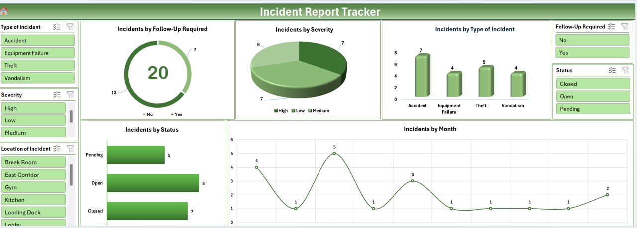
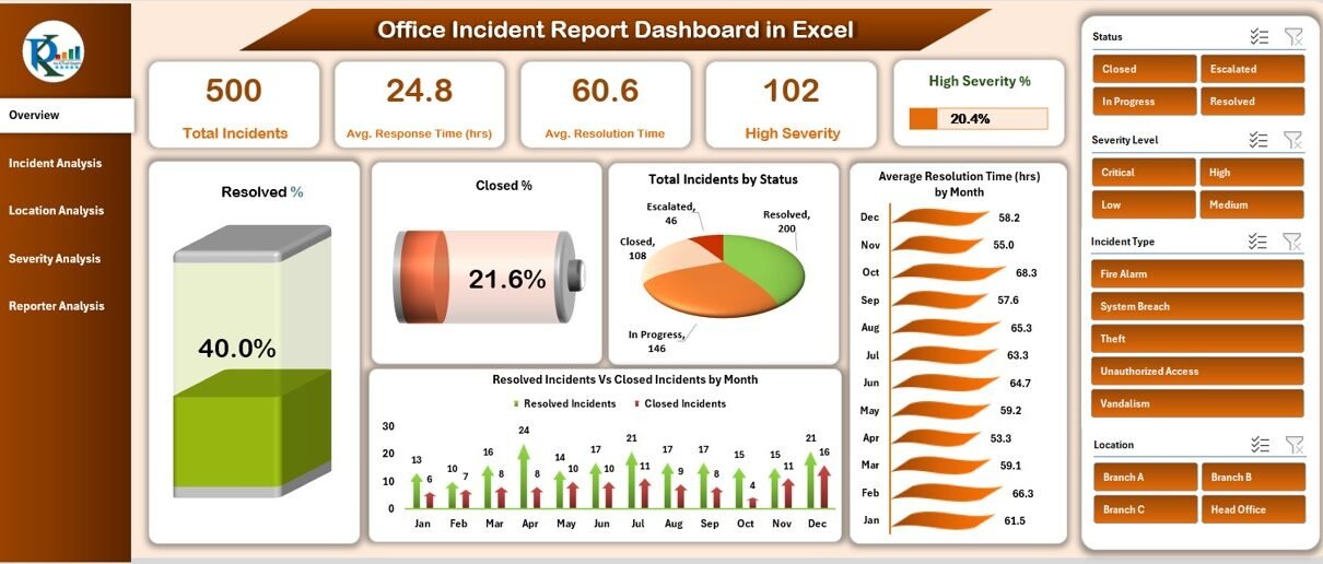
Take a look at these examples. This is the type of professional dashboard we are aiming to create.
1. Planning and Setting Up Your Dashboard
A good dashboard is well-planned. The goal is to present the most important information clearly, without overwhelming the user. A common best practice is to place high-level KPIs at the top, key charts in the main body, and interactive controls (like filters) to the side.
Let's avoid some common design mistakes from the start.
Excel Dashboards Guide: How to Build Interactive Reports
This guide from ASK Training highlights common mistakes in dashboard design. Reading this will help you think like a professional and create a report that is clear and easy to use.
Read the section titled 'Dashboard Design Mistakes to Avoid'. Pay close attention to the points about avoiding clutter ('Everything but the Kitchen Sink') and inconsistent formatting. We will apply these principles today.
Now, let's set up the canvas:
- Create a new sheet in your workbook and name it
Dashboard. - Go to the View tab and uncheck Gridlines and Headings. This immediately gives the sheet a cleaner, more report-like appearance.
- You can optionally set a background color for the entire sheet (e.g., a light grey or dark blue) by selecting all cells (
Ctrl+A) and using the Fill Color tool on the Home tab.
2. Creating Key Performance Indicator (KPI) Tiles
The KPIs on your Summary sheet (Total Incidents, Open Incidents, etc.) need to be displayed prominently. We'll create "KPI tiles" at the top of our dashboard using shapes and linked text boxes.
The video below demonstrates this technique clearly. You will add a shape for the background and then place a text box on top, which you will dynamically link to a cell in your Summary sheet.
Make a Dynamic Task Management Tracker in Excel!
The video from Kenji Explains shows how to build a dashboard from scratch. We will focus on the part where he creates the KPI tiles at the top.
Watch the segment from 08:28 to 10:20. In this part, he creates the text boxes and then, crucially, links them to the calculation cells using the formula bar (e.g., typing = in the formula bar and clicking the cell). This is the exact method you will use to display your KPIs.
Your Steps:
- On the
Dashboardsheet, go to Insert > Shapes and choose a shape (like a Rounded Rectangle). Draw one for your first KPI, "Total Incidents". Format its color as you like. - Go to Insert > Text Box and draw it on top of the shape.
- With the text box selected, click in the Formula Bar, type
=, navigate to yourSummarysheet, and click the cell containing the value for "Total Incidents". Press Enter. - Format the text (font size, color, alignment) to make it stand out.
- Add another text box for the label (e.g., "Total Incidents").
- Group the shape and text boxes together (select them all, right-click > Group).
- Duplicate this group for your other main KPIs: Open Incidents, Resolved Incidents, and Average Resolution Time. Remember to update the formula link for each new text box.
3. Building Interactive Charts with PivotCharts
While our Summary sheet is great for high-level numbers, we need more detailed, filterable visuals. The best way to do this is with PivotCharts. A PivotChart is a chart linked to a PivotTable, which allows it to be controlled by Slicers.
We'll create a few PivotTables from our main IncidentLog table to generate charts for:
- Incidents by Status
- Incidents by Priority
- Incidents by Owner
The following video from Kevin Stratvert is an excellent, comprehensive guide to this entire process. We will break it down into manageable steps.
📊 How to Build Excel Interactive Dashboards
This video from Kevin Stratvert is a masterclass in building interactive dashboards using PivotTables and Slicers. It covers the exact workflow we need to follow.
First, watch from 03:01 to 07:11. This section demonstrates the core process: Creating a PivotTable on a new sheet. Configuring the PivotTable fields (e.g., putting Country in Rows, Product in Columns, Profit in Values). Inserting a PivotChart from the PivotTable. Cleaning up the chart (e.g., adding a title, removing field buttons). You will follow this same process for each of your charts.
Your Steps:
- Create a new sheet and name it
DashboardCalcs. This will keep your workbook tidy by holding the PivotTables that power your dashboard. - Chart 1: Incidents by Status
- Click anywhere inside your
IncidentLogtable. - Go to Insert > PivotChart.
- In the dialog box, choose to place the PivotTable on your
DashboardCalcssheet. - In the PivotTable Fields pane, drag
Statusto the Rows (or Axis) area andIncidentIDto the Values area. Ensure it's set to "Count of IncidentID". - Choose a chart type (a Pie or Donut chart works well here).
- Clean up the chart: Add a title "Incidents by Status" and hide the field buttons (Right-click a button > "Hide all field buttons on chart").
- Click anywhere inside your
- Chart 2 & 3: By Priority and By Owner
- Repeat the process above to create two more PivotCharts on your
DashboardCalcssheet:- Incidents by Priority: Use
Priorityin Rows andCount of IncidentIDin Values. A Bar chart is a good choice. - Incidents by Owner: Use
Ownerin Rows andCount of IncidentIDin Values. A Bar chart is also suitable here.
- Incidents by Priority: Use
- Repeat the process above to create two more PivotCharts on your
- Move Charts to the Dashboard:
- Select each chart one by one, cut it (
Ctrl+X), and paste it (Ctrl+V) onto yourDashboardsheet. Arrange them below your KPI tiles.
- Select each chart one by one, cut it (
4. Making the Dashboard Interactive with Slicers
This is where the magic happens. Slicers are user-friendly filter buttons that can control multiple PivotCharts at once.
📊 How to Build Excel Interactive Dashboards
Let's return to Kevin Stratvert's video to see how to add Slicers and, most importantly, connect them to all of your charts.
Watch the final crucial steps from 12:51 to 16:05. This covers: Inserting Slicers (12:51 - 14:43): How to select a PivotChart and add Slicers for different fields. Connecting Slicers (14:43 - 16:05): This is the most important part. He shows you how to right-click a slicer, go to 'Report Connections', and link it to all the PivotTables you've created. This ensures that one click filters everything.
Your Steps:
- Click on any of your PivotCharts on the
Dashboard. - Go to the PivotChart Analyze tab and click Insert Slicer.
- In the dialog box, check the boxes for
Priority,Status, andOwner. Click OK. - Arrange the three new Slicer objects on your dashboard, perhaps on the left or right side.
- For each slicer:
- Right-click the slicer and choose Report Connections.
- In the pop-up window, you will see all the PivotTables you created. Check all the boxes to connect the slicer to every chart.
- Click OK.
Now, test it out! Click on a priority, status, or owner in a slicer. All of your charts should update instantly.
Your Turn: Assemble the Final Dashboard
You now have all the components. It's time to put them together into a polished, one-page report.
- Open your Incident Management Excel file which contains the
IncidentLogandSummarysheets. - Create the
DashboardandDashboardCalcssheets. Set up theDashboardsheet by removing gridlines. - Build the KPI Tiles: Create at least four tiles at the top of your
Dashboardfor Total, Open, and Resolved Incidents, and Average Resolution Time. Link them to yourSummarysheet. - Create the PivotCharts: On your
DashboardCalcssheet, create three PivotCharts based on yourIncidentLogdata:- Incidents by Status (Pie or Donut chart).
- Incidents by Priority (Bar chart).
- Incidents by Owner (Bar chart).
- Move and Arrange: Cut and paste your charts onto the
Dashboardsheet. Arrange them neatly below the KPI tiles. Use the alignment tools (Shape Format > Align) to ensure they are perfectly lined up. - Add and Connect Slicers: Insert slicers for
Priority,Status, andOwner. Position them on your dashboard and use Report Connections to link each slicer to all three of your PivotTables. - Final Polish: Adjust colors, fonts, and sizes to create a visually appealing and professional-looking dashboard. Ensure everything fits on one screen without scrolling.
Conclusion
Congratulations! You have successfully constructed a fully interactive, one-page dashboard. You've combined several powerful Excel features—Tables, COUNTIFS, PivotTables, PivotCharts, and Slicers—to build a professional-grade reporting tool. This ability to transform raw data into actionable, visual insights is a core skill for any MIS Executive.
In our final lesson for this capstone project, we will focus on using this system for ongoing reporting. You will learn how to prepare a weekly incident summary report by refreshing the data and extracting key insights, putting your new dashboard to practical use.