After-Tax Project Evaluation with Depreciation

Hello! Welcome back to our capstone module.

In our last session, we walked through a high-level, comprehensive analysis of a multi-alternative project, from initial framing to a final recommendation. We saw that a crucial step in that process was moving from a pre-tax to an after-tax analysis.

Today's lesson will focus entirely on that critical step. Our learning outcome is to integrate after-tax considerations and depreciation into a project evaluation. While a pre-tax analysis can be a quick filter, it's the after-tax analysis that reflects the true economic reality of an investment. For a manager evaluating significant technology projects, mastering this is non-negotiable for making sound financial decisions.

We will cover:

The fundamental mechanics of calculating After-Tax Cash Flow (ATCF).
How to calculate depreciation using the MACRS method, the standard for most US-based technology assets.
How to apply these concepts in a complete project evaluation.
Specific applications relevant to your work, including R&D tax credits and lease-vs-buy decisions.

1. The Core of After-Tax Analysis

An after-tax analysis correctly models two key realities:

Profits and savings are taxed, reducing the cash available to the company.
Depreciation, while a non-cash expense, creates a "tax shield" by reducing taxable income, which in turn reduces the taxes paid and thus increases the cash available.

The most straightforward way to calculate the After-Tax Cash Flow (ATCF) for any given year is with a two-step process:

Calculate Taxable Income (TI):
$T I = Before-Tax Cash Flow (BTCF) - Depreciation (D)$
- BTCF includes all cash inflows (revenues, savings) and cash outflows (operating costs, maintenance) for the period.
- Depreciation (D) is the allowable depreciation charge for the period.
Calculate After-Tax Cash Flow (ATCF):
$A T C F = B T C F - (T I \times t)$
- Where t is the corporate income tax rate.

This process is typically laid out in a table, year by year, to build a complete after-tax cash flow stream for the project.

Projected Cash Flow Statement Example — This real-world cash flow statement illustrates the concept. To get from 'Net Income' to 'Cash Flows from Operating Activities,' you can see that 'Depreciation' is added back. This is because it was subtracted to calculate income and taxes, but it wasn't a real cash outflow.

The key to this calculation is determining the correct depreciation charge for each year.

2. The MACRS Depreciation Method

While several depreciation methods exist (like the Straight-Line method we saw in a previous lesson's example), for-profit companies in the U.S. must use the Modified Accelerated Cost Recovery System (MACRS) for tax purposes.

MACRS groups assets into property classes with predefined recovery periods. For example, computers, software, and light vehicles fall into the 5-year property class. It also uses a half-year convention, which assumes assets are placed in service in the middle of the first year. This means a 5-year property is actually depreciated over 6 calendar years.

The following video provides a clear explanation of how to use the MACRS tables to find the correct depreciation percentage for each year.

How to Implement MACRS Depreciation Method + Example

To understand how to calculate depreciation for your projects, please watch this video on the MACRS method. It will walk you through the core concepts and show you how to apply the standard IRS tables.

Please watch the segments covering the MACRS assumptions (0:00-3:08), how to use the percentage tables (6:00-7:10), and the worked example (8:05-9:34). Focus on understanding the role of property classes and the half-year convention.

Test your understanding!

Your company buys a new server for $50,000. Servers are classified as 5-year MACRS property. Using the MACRS GDS Half-Year Convention table (which the video references), what would be the depreciation deduction for Year 1 and Year 2?

MACRS 5-Year Property Percentages:

Year 1: 20.00%
Year 2: 32.00%
Year 3: 19.20%
...and so on.

Show answer

Year 1 Depreciation: $50,000 * 20.00% = $10,000
Year 2 Depreciation: $50,000 * 32.00% = $16,000

Notice how the depreciation is "accelerated"–you get larger deductions in the earlier years, which is financially beneficial due to the time value of money.

3. A Complete After-Tax Project Evaluation

Now, let's integrate these concepts into a full Present Worth (PW) analysis. The following video works through a complete problem, from initial costs to a final investment decision, all on an after-tax basis.

While this example uses the simpler straight-line depreciation method to illustrate the concepts, the process is identical if you substitute MACRS depreciation values.

Present Worth of After Tax Cash Flows of an Investment - Engineering Economics Lightboard

This video from the Engineering Economics Guy will walk us through a full after-tax analysis. It masterfully demonstrates how each component of a project—initial cost, savings, and salvage value—is affected by taxes.

Please watch the entire video. Pay close attention to these three key calculations: The tax shield from depreciation (explained starting around 05:05): Notice how the initial cost generates future tax savings. After-tax operating savings (starting at 09:17): The recurring annual savings are reduced by taxes. After-tax salvage value (starting at 11:02): The cash received from selling the asset is also taxed.

To summarize the logic from the video and our formulas:

Cash Flow Component	Before-Tax Value	After-Tax Treatment
Initial Cost	-P	-P (This is a cash outflow at time 0)
Depreciation Tax Shield	N/A	A stream of positive cash flows equal to $D_{k} \times t$ for each year k. The video calculates the PV of this stream.
Annual Savings	+S	+S(1 - t). An annuity of after-tax savings.
Salvage Value	+SV	+SV - (SV - BV) $\times$ t, where BV is the book value at the time of sale. If BV=0, this simplifies to SV(1-t).

By finding the present worth of each of these after-tax components and summing them up, you arrive at the project's after-tax Net Present Worth (NPW).

4. Applications for Technology & Software Projects

Your background as a software leader opens up specific and high-value applications of after-tax analysis.

R&D Tax Credits for Software Development

Many software development activities don't just generate depreciation; they can qualify for R&D Tax Credits. A tax credit is a dollar-for-dollar reduction of your tax bill, making it far more valuable than a deduction.

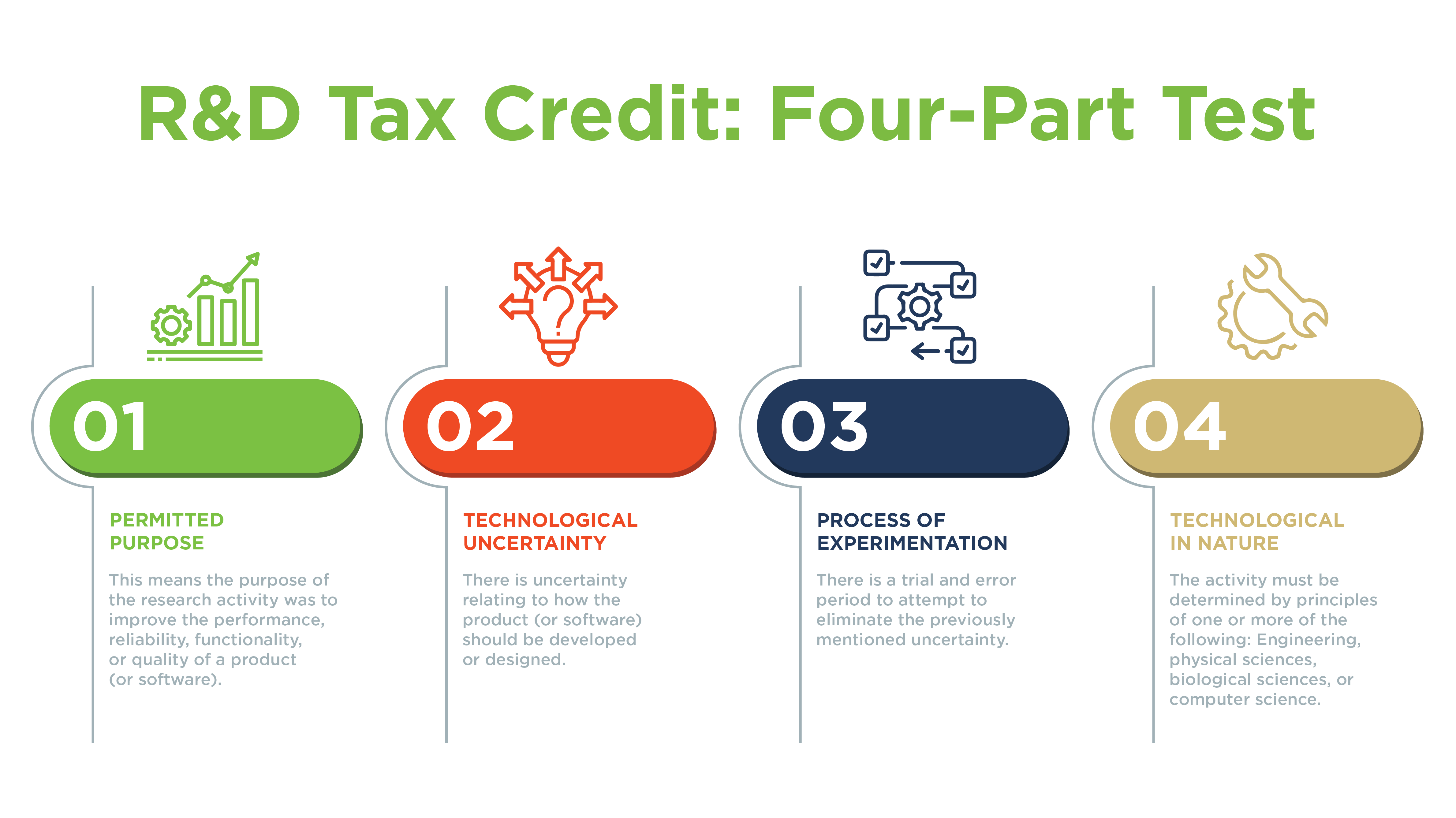
R&D Tax Credit: Four-Part Test — This diagram shows the four criteria an activity must meet to qualify for R&D tax credits. As you can see, activities aimed at improving software performance or functionality by resolving technological uncertainty through experimentation often qualify. This is a powerful financial lever in software-intensive companies.

When evaluating a project, if you anticipate that some development costs will generate R&D credits, those credits should be included in your ATCF calculation as a direct cash inflow (or reduction of outflow) in the year they are claimed.

Lease vs. Purchase Decisions

A classic dilemma for technology infrastructure is whether to buy servers or lease them from a cloud provider (e.g., AWS, Azure). An after-tax analysis is the only way to compare these two options properly because their tax treatments are completely different.

Lesson 9: After-Tax Decision Methods and Applications

To understand the financial difference between leasing and buying, it's helpful to see how their cash flows are structured. Please read the introduction to this topic from Penn State's course materials.

Read the section titled 'Lease versus Purchase'. Focus on the introductory paragraphs and the summary comparison between an 'Operating Lease' and 'Capital Lease'. This will clarify why the tax implications are so different.

Here's the essential difference for an Operating Lease (the common model for cloud services):

Purchase Alternative: You pay the capital cost upfront, and you get to claim depreciation deductions over the asset's life.
Lease Alternative: You have no upfront capital cost. The periodic lease payments are treated as an operating expense and are fully deductible from taxable income. You do not claim depreciation.

This creates a fascinating trade-off between a large upfront cost with future depreciation shields versus a steady stream of tax-deductible rental payments. The superior choice can only be found by building an ATCF model for each alternative and comparing their NPW or equivalent annual worth.

Conclusion

You've now added the final layer of realism to project evaluation. By moving from a pre-tax to an after-tax world, your analysis becomes a far more accurate predictor of a project's true financial impact.

Key Takeaways:
- After-Tax Cash Flow (ATCF) is calculated by taking Before-Tax Cash Flow (BTCF) and subtracting the taxes owed.
- Taxes are calculated on Taxable Income, which is BTCF minus the allowable depreciation charge (TI = BTCF - D).
- For U.S. companies, depreciation for tax purposes is typically calculated using the MACRS method.
- A full after-tax evaluation requires building a year-by-year cash flow table that correctly models the tax effects of revenues, operating costs, depreciation, and salvage value.
- For technology projects, special considerations like R&D tax credits and lease-vs-purchase tax treatments are critical.

Preview of the Next Lesson

We have now constructed a robust after-tax model of a project. But this model is built on assumptions—about revenues, costs, and other variables. In our next lesson, we will learn how to incorporate sensitivity analysis to assess the impact of uncertainty on a project recommendation. This will allow us to stress-test our conclusions and identify the most critical risks to a project's success.

Recommended resources