Software Make-vs-Buy: Present Worth Analysis

Hello! Welcome to our next lesson.

In our last few sessions, we've built a solid understanding of Present Worth (PW) analysis, learning how to compare alternatives and account for end-of-life costs like salvage values and disposal fees. Now, we'll apply this powerful tool to one of the most common and critical decisions in the technology industry.

Your learning outcome for this lesson is to evaluate make-vs-buy decisions for software components using present worth analysis. As an experienced software developer and manager, you've undoubtedly been part of conversations about whether to build a feature from scratch or integrate a third-party solution. This lesson will provide a structured, quantitative framework to support those decisions, moving from gut feeling to data-driven analysis.

Framing the Make-vs-Buy Decision

The "make-vs-buy" choice is a classic business strategy problem. In software engineering, it manifests as the decision between:

Make (Build): Developing a software component, module, or system in-house using your own team's resources.
Buy: Acquiring the functionality from an external source. This can include:
- Purchasing a Commercial-Off-The-Shelf (COTS) product.
- Subscribing to a Software-as-a-Service (SaaS) platform.
- Integrating an open-source library (which may still have associated support or maintenance costs).
- Outsourcing the development to a third-party vendor.

Each path has a distinct profile of costs and benefits. Our goal is to translate these into cash flows and compare them on an equal footing using Present Worth analysis.

Identifying the Cash Flows

To perform a PW analysis, we first need to identify the relevant cash flows for each alternative over a chosen study period (e.g., 5 years).

Cost Category	Make (Build) Alternative	Buy Alternative
Initial Costs (Outflows)	• Development Costs: Salaries for developers, QAs, PMs; tools; initial infrastructure setup. • Opportunity Cost: What other projects could the team be working on? (This is often captured by ensuring the project's return meets the MARR).	• Acquisition Costs: License fees, purchase price. • Integration Costs: Labor required to integrate the component into your existing systems. • Initial Setup/Training Costs: Getting the team up to speed.
Recurring Costs (Outflows)	• Maintenance: Bug fixes, security patches, refactoring. • Support: Time spent helping internal or external users. • Infrastructure: Ongoing server or hosting costs.	• Subscription/License Fees: Annual or monthly payments. • Maintenance/Support Contracts: Annual fees for vendor support and updates. • Usage-based Costs: Fees per user, per API call, etc.
End-of-Life (In/Outflows)	• Salvage Value: (Rare) If the component can be sold or licensed to others. • Disposal/Decommissioning: Costs to retire the component securely.	• Usually none, unless there are costs associated with migrating data away from the vendor's platform.

An Example: The Cost Tradeoff

To see how these costs play out, let's look at a simple example. The following presentation slides discuss a make-or-buy decision for a Transaction Processing System (TPS).

Software Decision Analysis Techniques

These slides from a presentation on Software Engineering Economics lay out a make-vs-buy scenario. Focus on how the costs are broken down for the two alternatives.

Please review the three slides starting from the one titled 'COTS vs. New Development Cost Tradeoff: TPS II'. This includes a description of the problem, a table breaking down the costs, and a graph visualizing the tradeoff. Note how costs are categorized for 'COTS' (Buy) versus 'New Development' (Make).

The key takeaway from that example is how the decision hinges on a variable—in this case, the number of regional concentrators N. The graph shows a breakeven point where one option becomes cheaper than the other as the scale of the operation changes.

However, you might have noticed that the analysis simply sums the costs over the 5-year lifecycle. This is a common simplification, but it ignores the time value of money. A proper engineering economic analysis uses Present Worth to discount future costs, giving us a more accurate comparison.

Applying Present Worth Analysis: A Worked Example

Let's apply the rigorous PW method to a scenario you might encounter.

Scenario: Your company is launching a new SaaS product and needs an analytics dashboard. The team is deciding between building a custom dashboard or integrating a third-party service. The study period is 5 years and the company's MARR is 15%.

Option 1: Make (Build in-house)
- Upfront Development Cost: $120,000 (Year 0)
- Annual Maintenance & Server Costs: $20,000 (Years 1-5)
- Major Upgrade: A significant feature enhancement is planned for Year 3 at a cost of $40,000.
Option 2: Buy (Use "AnalyticsCorp" Service)
- Initial Integration & Setup Cost: $15,000 (Year 0)
- Annual Subscription Fee: $45,000 (Years 1-5)

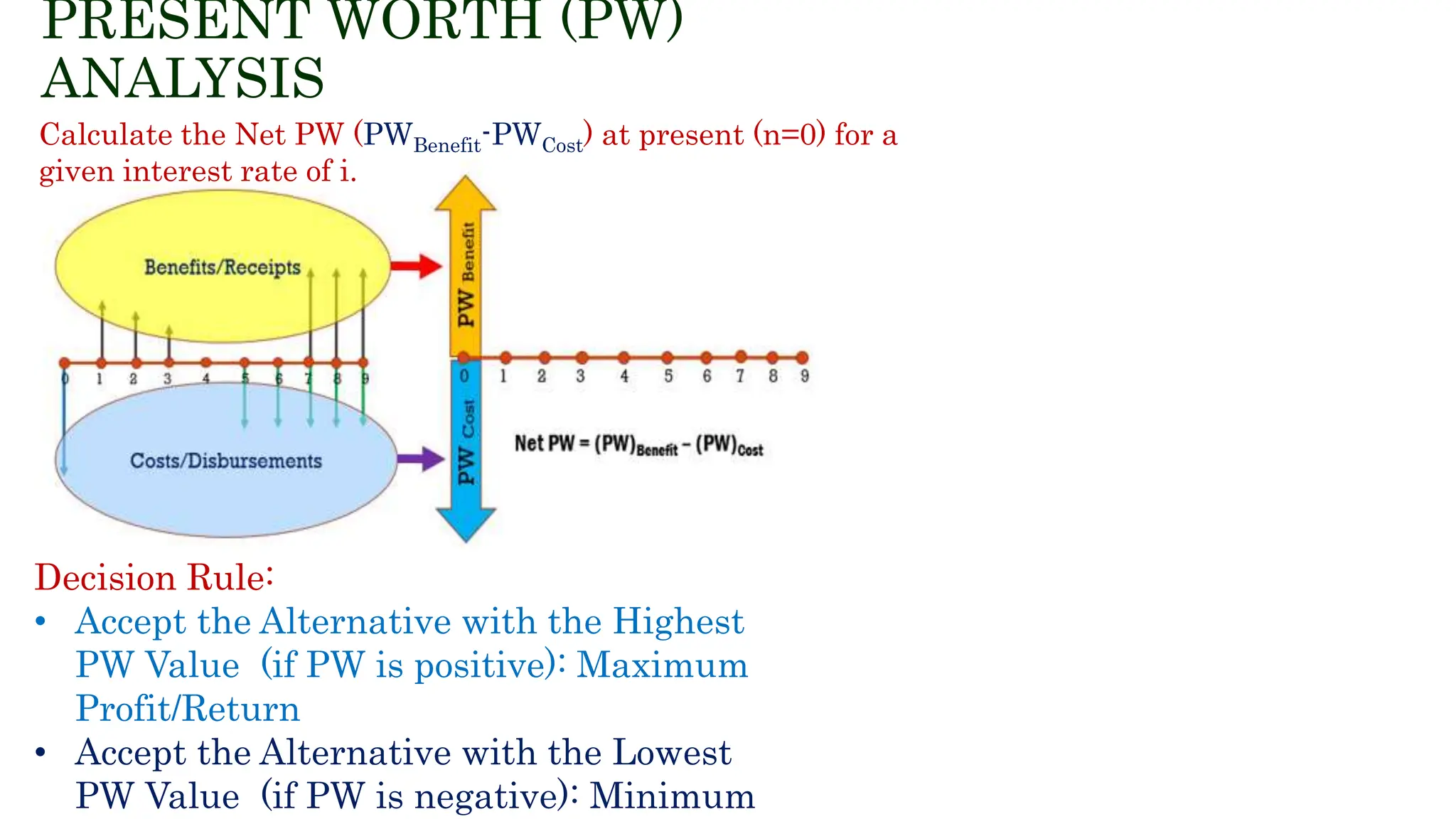
Our decision rule is to choose the alternative with the lower Present Worth of cost.

Present Worth Analysis Diagram and Decision Rule — As a refresher, this diagram shows the core principle of PW analysis: all future cash flows (both costs and benefits) are discounted back to time 0 to find a single Net Present Worth value for comparison.

Calculation:

We need to find the PW of each alternative's cost stream. We'll use the following factors:

(P/A, 15%, 5) = 3.3522
(P/F, 15%, 3) = 0.6575

1. Present Worth of "Make"
The cash flows are the initial development cost, the annual maintenance costs, and the upgrade cost in Year 3.

$P W_{M ak e} = - (Initial Cost) - (Annual Cost) (P / A, 15%, 5) - (Upgrade Cost) (P / F, 15%, 3)$
$P W_{M ak e} = - 120, 000 - 20, 000 (3.3522) - 40, 000 (0.6575)$
$P W_{M ak e} = - 120, 000 - 67, 044 - 26, 300$
$P W_{M ak e} = - $213, 344$

2. Present Worth of "Buy"
The cash flows are the initial setup cost and the annual subscription fee.

$P W_{B u y} = - (Initial Cost) - (Annual Cost) (P / A, 15%, 5)$
$P W_{B u y} = - 15, 000 - 45, 000 (3.3522)$
$P W_{B u y} = - 15, 000 - 150, 849$
$P W_{B u y} = - $165, 849$

Decision:
Comparing the two, PW_Buy (-$165,849) is less negative than PW_Make (-$213,344). Therefore, based purely on this economic analysis, buying the third-party service is the preferred alternative.

Test your understanding!

Your team needs a data scraping component for a project. You'll analyze the decision over a 4-year period with a MARR of 10%.

Make: Initial development cost of $50,000. Annual maintenance will cost $10,000.
Buy: An annual license for a scraping tool costs $20,000 per year, paid at the start of each year (i.e., years 0, 1, 2, 3). There is also a one-time $5,000 integration cost in Year 0.

Which option is economically better?
(Hint: For the "Buy" option, you have a cost at year 0 and a uniform series for years 1-3. Or, you can think of it as a $25,000 cost at year 0 and an annuity of $20,000 for years 1 through 4, then subtract the final payment. A simpler way is to treat it as a $25k cost at t=0 and an annuity of $20k for years 1-3.)
Let's use the annuity formula for years 0-3: P = A(P/A, i, n). A payment at the beginning of a period is an "annuity due". The formula is P = A[1 + (P/A, i, n-1)].
Factor values: (P/A, 10%, 4) = 3.1699, (P/A, 10%, 3) = 2.4869.

Show answer

1. Present Worth of "Make"
$P W_{M ak e} = - 50, 000 - 10, 000 (P / A, 10%, 4)$
$P W_{M ak e} = - 50, 000 - 10, 000 (3.1699)$
$P W_{M ak e} = - 50, 000 - 31, 699 = - $81, 699$

2. Present Worth of "Buy"
The costs are $25,000 at Year 0 ($5k integration + $20k first license payment) and then $20,000 at the start of years 1, 2, and 3. We can treat this as a $25k initial cost plus an annuity of $20k for years 1 through 3.
$P W_{B u y} = - 25, 000 - 20, 000 (P / A, 10%, 3)$
$P W_{B u y} = - 25, 000 - 20, 000 (2.4869)$
$P W_{B u y} = - 25, 000 - 49, 738 = - $74, 738$

Decision: The "Buy" option (PW = -$74,738) has a lower present worth of cost than the "Make" option (PW = -$81,699). Therefore, buying the tool is the more economical choice.

Beyond the Numbers: Strategic & Qualitative Factors

A PW analysis provides a crucial quantitative answer, but it's rarely the only factor. As a manager, you must also weigh qualitative aspects that are difficult to assign a dollar value to. The following document from Carnegie Mellon's Software Engineering Institute provides an excellent high-level perspective on this.

Investment Analysis of Software Assets for Product Lines

This report, 'Investment Analysis of Software Assets for Product Lines,' discusses the strategic thinking behind make-vs-buy decisions. It moves beyond simple cost calculations to consider risk, flexibility, and other critical business factors.

First, read the motivating example at the start of the introduction (from 'Suppose you are a manager...' to '...craft each product independently, lifting code from the previous release?'). Then, read the subsection titled 'Select Assets', which starts with 'Activity Costs'. Focus on the three key criteria discussed: Activity Costs, Asset Flexibility, and Skill.

Based on that reading and our discussion, always supplement your quantitative analysis by asking these strategic questions:

Time to Market: The "buy" option is almost always faster to implement, which could be a significant competitive advantage.
Strategic Control: Is this component a core part of your intellectual property and competitive advantage? If so, "making" it might be essential, even if it's more expensive.
Flexibility & Customization: Can the "buy" solution meet 100% of your requirements, both now and in the future? An in-house solution offers maximum flexibility.
Focus & Core Competency: Does building this component distract your team from its primary mission? It's often better to "buy" commodity functions (like payment processing or authentication) and "make" what is unique to your business.
Vendor Risk: What happens if the vendor for your "buy" solution goes out of business, gets acquired, or dramatically increases prices?
Team Skills: Do you have the necessary expertise to build and, more importantly, maintain the component?

Conclusion

You now have a complete framework for tackling make-vs-buy decisions for software components. It's a two-part process: first, a rigorous quantitative comparison using Present Worth analysis, followed by a thoughtful qualitative review of strategic factors.

Key Takeaways:
- Make-vs-buy decisions are a comparison of two mutually exclusive alternatives: building in-house or acquiring externally.
- The core of the quantitative analysis is to calculate the Present Worth of costs for each alternative over a defined study period.
- The alternative with the lower PW of costs (the less negative number) is the economically preferred choice.
- This numerical result must be balanced with critical qualitative factors like strategic control, time-to-market, and flexibility.

Preview of the Next Lesson

In our next lesson, we will apply the present worth method to build-vs-lease decisions for technology infrastructure. You'll see that it's a very similar type of problem. Instead of a software component, we'll be evaluating physical hardware or cloud services. The decision is whether to "build" your own on-premise data center or "lease" capacity from a cloud provider like AWS or Azure. The analytical method you learned today will apply directly.

Recommended resources