Present Value of Arithmetic Gradient Series

What is an Arithmetic Gradient Series?

An arithmetic gradient series is a sequence of cash flows that increases or decreases by a constant amount from one period to the next. This constant amount is called the gradient, denoted by $G$.

• If $G$ is positive, it's an increasing gradient. Think of rising maintenance costs for aging equipment.
• If $G$ is negative, it's a decreasing gradient. Imagine the declining revenue from an older software product as it's phased out.

To see some practical applications of this concept, let's watch the beginning of the following video.

The Core Strategy: Decomposition

The key to analyzing an arithmetic gradient series is to break it down into two simpler components that we can work with:

1. A Uniform Series (Annuity), which we'll call $A$. This represents the constant base amount of the cash flow.
2. A Pure Gradient Series, which starts at zero in period 1 and increases or decreases by the gradient amount $G$ in each subsequent period.

This decomposition is the most important part of the process.

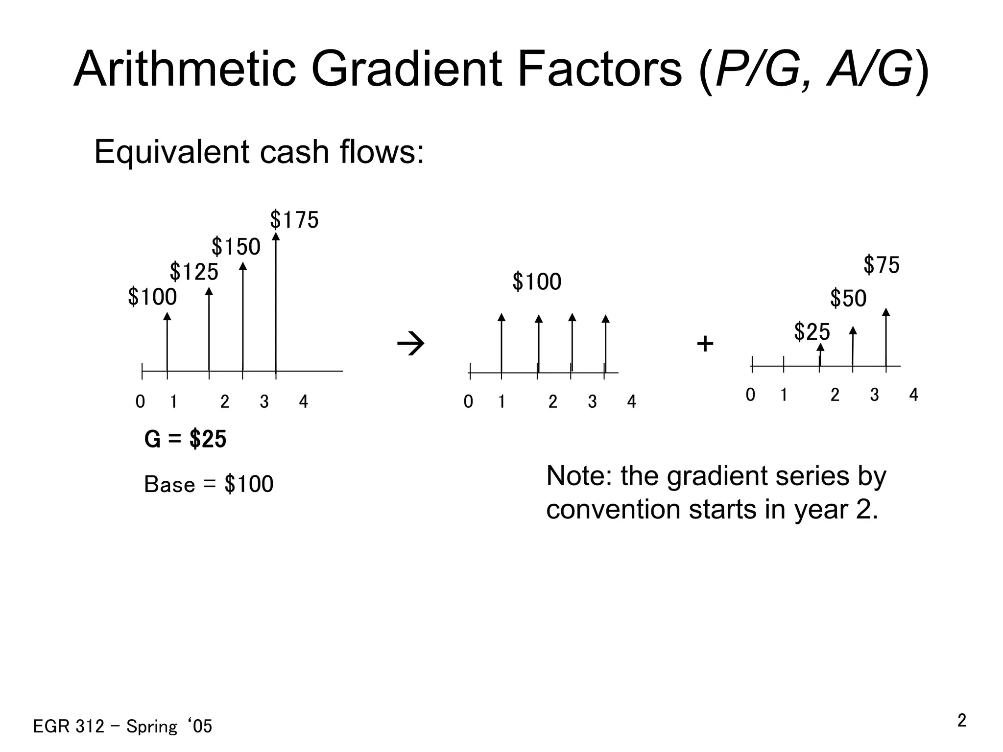
The total present worth ($P_T$) of the entire series will be the sum of the present worth of the uniform series ($P_A$) and the present worth of the pure gradient series ($P_G$):

$P_T=P_A+P_G$

Calculating the Present Value

We already know how to calculate $P_A$ from our previous lessons:

$P_A=A(P/A,i,n)$

To find $P_G$, we introduce a new factor: the arithmetic gradient present worth factor, denoted as (P/G, i, n). This factor converts a pure gradient series with increment $G$ into its equivalent present value at time 0.

The complete formula for the total present worth is:

$P_T=A(P/A,i,n)+G(P/G,i,n)$

Let's apply this to a practical example relevant to your software background.

Example: Escalating Maintenance Contract

Imagine your company is signing a 5-year maintenance contract for a critical on-premise database.

• The cost in Year 1 is $20,000.
• The vendor anticipates that due to aging hardware and increasing complexity, the cost will increase by $3,000 each year.
• Your company's MARR is 12%.

What is the total Present Worth (PW) of this contract's costs?

Step 1: Identify the components.

• The cash flow in Year 1 defines the base annuity: $A=\$20,000$.
• The constant annual increase is the gradient: $G=\$3,000$.
• The interest rate is $i=12\%$.
• The number of periods is $n=5$.

Step 2: Decompose the cash flow.
The contract is equivalent to:

• A uniform series of $20,000 per year for 5 years.
• A pure gradient series starting at Year 2 with $3,000, increasing by $3,000 each year for 5 years.

Step 3: Find the values for the P/A and P/G factors.
You can find these in interest tables or use their formulas. Given your software engineering background, you might appreciate seeing the underlying formulas:

• P/A factor formula: $(P/A,i,n)=\frac{(1+i{)}^n-1}{i(1+i{)}^n}$
• P/G factor formula: $(P/G,i,n)=\frac{(1+i{)}^n-in-1}{i^2(1+i{)}^n}$

For $i=12\%$ and $n=5$:

• $(P/A,12\%,5)=3.6048$
• $(P/G,12\%,5)=6.3970$

Step 4: Calculate the Present Worth of each component and sum them.

• $P_A=A(P/A,12\%,5)=\$20,000\times 3.6048=\$72,096$
• $P_G=G(P/G,12\%,5)=\$3,000\times 6.3970=\$19,191$
• $P_T=P_A+P_G=\$72,096+\$19,191=\$91,287$

So, the equivalent cost of this 5-year contract at today's value is $91,287.

The following image provides a concise visual summary of this combined calculation process.

To see another full walkthrough of this decomposition and calculation, please review the following resource.

Handling Decreasing Gradients

What if the cash flows are decreasing? The logic is identical, but the gradient $G$ is negative.

For instance, consider a machine that saves your company $28,000 in labor costs in its first year. As the machine wears and becomes less efficient, the savings decrease by $2,000 per year over its 6-year life. To find the present worth of these savings, you would set $A=\$28,000$ and $G=-\$2,000$. The calculation would be:

$P_T=A(P/A,i,n)+(-\$2,000)(P/G,i,n)$

The negative gradient component reduces the total present worth of the base annuity. The resource below provides an excellent example of this.

Conclusion

You have now added another essential tool to your engineering economics toolkit. You can move beyond simple uniform cash flows and model scenarios where costs or benefits change linearly over time.

• Key Takeaways:
  • An arithmetic gradient series involves cash flows that change by a constant amount ($G$) each period.
  • The standard method for analysis is to decompose the series into a base uniform series ($A$) and a pure gradient series ($G$).
  • The total present worth is found by summing the present worth of each component: $P_T=A(P/A,i,n)+G(P/G,i,n)$.
  • This method works for both increasing ($+G$) and decreasing ($-G$) gradients.

Preview of the Next Lesson

We've now covered constant payments (uniform series) and linearly changing payments (arithmetic gradient). But what about situations where things change by a constant percentage? Think of revenue that grows by 5% per year. For this, we need a different tool. In our next lesson, we will explore the geometric gradient series.