Hello! Welcome back to your course on Engineering Economics.
In our last lesson, we established a formal way to talk about uncertainty by using the language of probability. We learned about sample spaces, events, and the fundamental axioms that govern how we assign likelihoods to different outcomes. You saw that for a project with uncertain revenues, we could model this with probabilities for "Low," "Medium," and "High" demand scenarios.
However, a list of probabilities and outcomes doesn't tell us which project to choose. Today, we bridge that gap. This lesson directly addresses the learning outcome: to calculate and interpret the expected value for projects with probabilistic outcomes. We will learn how to synthesize all the possible outcomes and their likelihoods into a single, powerful number that can guide our investment decisions. This is the cornerstone of making rational choices in the face of uncertainty.
1. Defining Expected Value: The "Long-Run Average"
Imagine you're evaluating a new feature for your platform. There's a chance it's a huge hit, a chance it's a moderate success, and a chance it flops. If you could somehow run this "experiment" a thousand times, what would be the average profit you'd make per attempt? This is the core intuition behind Expected Value.
To get a formal introduction to this concept, let's turn to the MIT OpenCourseWare materials.
This video, 'L05.8 Expectation', introduces the concept of expected value, starting with an intuitive example of a game of chance and then providing the formal definition. It perfectly explains how we arrive at a single number to summarize a random variable.
Please watch from the beginning until the timestamp 03:39. Focus on how the idea of 'average gain' in a game played many times leads directly to the formula for expected value.
As the video explains, the expected value is a weighted average of the outcomes, where the weights are the probabilities of those outcomes occurring.
The formal definition for a random variable that can take on values with corresponding probabilities is:
This is also often denoted by (mu).
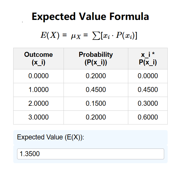
A crucial point of interpretation: The expected value is not necessarily a value you expect to see in any single trial. In the video's game, the possible outcomes were $1, $2, and $4, but the expected value was $2.70. Rather, it represents the average result if the experiment were repeated over and over.
2. Application: Expected Monetary Value (EMV) in Project Decisions
In engineering economics, our outcomes are typically financial—costs, revenues, or profits. When the random variable represents monetary amounts, its expected value is called the Expected Monetary Value (EMV). This is the tool we use to compare uncertain projects.
Let's watch a practical example that should resonate with your background in product development.
Decision Tree Analysis - Intro and Example with Expected Monetary Value
This video, 'Decision Tree Analysis - Intro and Example with Expected Monetary Value', walks through a classic business decision: choosing which of two products to invest in. It demonstrates precisely how to calculate and use EMV to make a rational choice.
Please watch the entire video. Pay close attention to how the development cost, probabilities of success and failure, and potential gains/losses are combined to calculate the EMV for both Product A and Product B.
This example beautifully illustrates why a simple analysis can be misleading. Product B had a higher potential payoff ($900 vs. $700), but its higher development cost and different risk profile made it the inferior choice. The EMV calculation provided the correct decision guidance.
- Decision Rule: When comparing mutually exclusive projects, choose the one with the higher (or less negative) Expected Monetary Value.
Test your understanding!
You are deciding between two strategies for implementing a new API for your platform.
-
Strategy A: Use a 3rd Party Service. This has a low initial cost. Your analysis shows:
- A 70% probability of low user traffic, resulting in a net profit of $100,000.
- A 30% probability of high user traffic (triggering high API fees), resulting in a net profit of $20,000.
-
Strategy B: Build the API In-House. This has a high initial development cost but better performance, which might attract more users. Your analysis shows:
- A 50% probability of high user adoption, resulting in a net profit of $150,000.
- A 50% probability of low user adoption, resulting in a net loss of -$30,000.
Calculate the EMV for both strategies. Which one should you choose and why?
Show answer
Let's calculate the EMV for each strategy:
Strategy A (3rd Party):
EMV(A) = (0.70 * $100,000) + (0.30 * $20,000)
EMV(A) = $70,000 + $6,000
EMV(A) = $76,000
Strategy B (In-House):
EMV(B) = (0.50 * $150,000) + (0.50 * -$30,000)
EMV(B) = $75,000 - $15,000
EMV(B) = $60,000
Decision: You should choose Strategy A.
Reasoning: The Expected Monetary Value of Strategy A ($76,000) is higher than that of Strategy B ($60,000). Although building the API in-house has a higher potential upside ($150k), it also carries a significant risk of a loss, which makes its probability-weighted average outcome less attractive than the safer third-party strategy.
3. Properties of Expected Value
To round out our understanding, it's useful to know a few key mathematical properties of expected value. These will become very helpful as we analyze more complex models. The MIT course readings provide a concise summary.
18.05 S22 All Probability Reading
The provided reading, '18.05 S22 All Probability Reading', contains a section dedicated to Expected Value that details its formal properties. We'll focus on the most important one: linearity.
From the document, please navigate to the sub-reading titled 'Discrete Random Variables: Expected Value'. Read the section '2.2 Algebraic properties of E[X]' (page 3 of that sub-reading). Focus on understanding the two properties listed, especially the first one regarding the sum of random variables.
The most critical property discussed is linearity. In simple terms:
- The expected value of a sum is the sum of the expected values:
- Constants can be factored out:
The first property is incredibly powerful. As your reading shows with the binomial example, if you want the expected number of successes in trials, you don't need to do a complex summation. You can just find the expected value of one trial () and multiply it by . This is analogous to how in software development, you can often analyze the performance of a simple, repeatable unit of code and then scale that analysis up, rather than analyzing the entire complex loop at once.
Conclusion
Today, you've learned to wield one of the most fundamental tools for decision-making under uncertainty. By calculating a project's expected value, you can move beyond gut feelings and simple "best-case/worst-case" thinking.
- Key Takeaways:
- Expected Value is the probability-weighted average of all possible outcomes of an uncertain event.
- Expected Monetary Value (EMV) is the application of this concept to financial outcomes, providing a single metric to compare risky projects.
- The rational decision rule is to select the alternative with the most favorable EMV.
- Expected value is a linear operator, meaning , which simplifies the analysis of complex systems.
Preview of the Next Lesson
The EMV is perfect for a single-stage decision. But what if a project involves a sequence of choices? For example: "Should we build a prototype? If the prototype is successful, should we launch a full product? If we launch, what marketing budget should we choose?"
In our next lesson, we will introduce Decision Trees. This is a powerful visual method for mapping out these sequential decisions and chance events. You'll see that the EMV we learned to calculate today is the engine that drives the analysis of these more complex, multi-stage problems.