Hello! Welcome to the first lesson in our new unit on the Determination of Income and Employment. We've successfully covered Money and Banking, and now we're diving into what is arguably the most important unit in Macroeconomics for your board exams, especially for numerical questions.
Today's lesson lays the essential groundwork. We will explore the concept of Aggregate Demand (AD). By the end of our 60 minutes, you will be able to explain what AD is and describe its components, specifically Consumption (C) and Investment (I), within the context of a simplified two-sector model. Mastering this foundation is the first step to confidently tackling the numerical problems in this chapter.
1. What is Aggregate Demand?
Just as you study the demand for a single product in microeconomics, in macroeconomics, we look at the total demand for all final goods and services in the entire economy. This is called Aggregate Demand.
Let's begin with a video that defines AD and introduces its various components.
Aggregate demand and related concepts | Macroeconomics | Class 12 | chapter 7 | Part 1
The video "Aggregate demand and related concepts" by Rajat Arora provides a clear and exam-oriented introduction to this topic.
Please watch the first part of the video from the definition of AD. Pay close attention to these points: The formal definition of Aggregate Demand (AD) as the total value of final goods and services all sectors in an economy are planning to buy. The idea that AD is equal to Aggregate Expenditure (AE). The four components of AD in an open, four-sector economy: Private Consumption Expenditure (C) Investment Expenditure (I) Government Expenditure (G) Net Exports (X-M) The connection between these components and the Expenditure Method of calculating National Income, which you've studied earlier. After this, watch the brief clarification from this segment on why AD is considered a flow concept.
2. The Two-Sector Model: Simplifying AD
For the purpose of your Grade 12 syllabus, the analysis of income determination is simplified to a two-sector closed economy, which consists of only households and firms. This means we will ignore the government (G) and the foreign sector (Net Exports, X-M) for now.
In this simplified model, Aggregate Demand has only two components:
AD = C + I

The video you just watched confirms this simplification. The instructor explicitly states that while AD has four components in theory, the syllabus focuses on the two-sector model. Let's hear him explain it.
Aggregate demand and related concepts | Macroeconomics | Class 12 | chapter 7 | Part 1
Continuing with the same video by Rajat Arora.
Watch the short segment from this clip, where he clarifies that for the rest of the chapter, we will consider AD = C + I.
3. The Components: Consumption (C) and Investment (I)
Now, let's look closer at C and I in our model.
Consumption (C): This is the planned expenditure by households.
- It is primarily dependent on income. As income rises, consumption also tends to rise.
- A crucial point is that consumption is never zero, even if income is zero. People need to consume to survive, and they do so by using past savings or by borrowing. This minimum level of consumption at zero income is called Autonomous Consumption (C̄).
Investment (I): This is the planned expenditure by firms on new capital goods (like machinery and buildings).
- In reality, investment depends on many factors like interest rates and business expectations.
- However, to keep our model simple, we will assume that investment is autonomous. This means it is a fixed amount that does not change when income changes. We denote it as Ī.
The best way to understand how these components come together is to see them in a table (schedule) and a graph.
Aggregate demand and related concepts | Macroeconomics | Class 12 | chapter 7 | Part 1
Let's return to the Rajat Arora video one last time. This part is crucial as it demonstrates how the AD curve is constructed from its components.
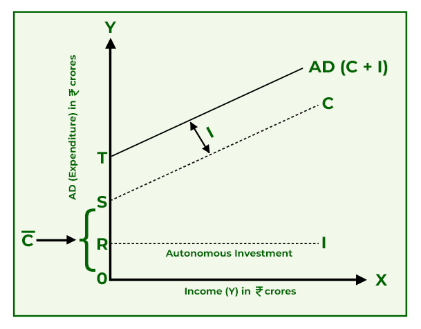
Watch from this detailed section. Focus on: How the consumption schedule is built, starting with autonomous consumption (C̄ = 40 in his example) at zero income. How the investment schedule is constant (Ī = 20) because it's autonomous. How the AD schedule is simply the sum of C and I at each income level. The graphical representation: The Investment curve (I) is a horizontal line. The Consumption curve (C) starts from the C̄ value on the Y-axis and slopes upwards. The AD curve starts from (C̄ + Ī) on the Y-axis and runs parallel to the C curve.
The graph you saw being constructed is a standard representation in macroeconomics.
4. Summary and Key Characteristics
To consolidate your understanding, let's review the main points about Aggregate Demand and its components in a clear, readable format.
Components of Aggregate Demand - GeeksforGeeks
This article from GeeksforGeeks, "Components of Aggregate Demand," provides a concise summary of the concepts we've discussed.
Please read the following sections: Start under the heading "Components of Aggregate Demand" and briefly review the four main components. Focus on the section "Aggregate Demand in a Two-Sector Model (AD = C + I)". Study the formula, the table, and the graph provided. Read the "Important Points About Aggregate Demand" at the end. This is an excellent summary of the key characteristics of the AD curve, such as the concept of Autonomous Consumption and why the AD curve has a positive slope and starts above the origin.
Conclusion
In this lesson, we've laid the critical foundation for the chapter on Income and Employment. You now understand the core concept of Aggregate Demand and how it is constructed in the simplified two-sector model that is central to your syllabus.
Key Takeaways:
- Aggregate Demand (AD) is the total planned expenditure on final goods and services in an economy.
- In a four-sector economy, AD = C + I + G + (X-M).
- For our analysis, we use a two-sector model, where AD = C + I.
- Consumption (C) has an autonomous component (C̄) that is independent of income and an induced component that depends on income.
- Investment (I) is assumed to be autonomous (Ī), meaning it's a constant value.
- The AD curve starts above the origin because of autonomous consumption and investment (C̄ + Ī), and it is positively sloped because consumption increases with income.
You've taken the first crucial step towards mastering the numericals of this unit. In our next lesson, we will delve deeper into the consumption and saving behavior of households. We will formally define the consumption function and saving function and introduce the important concepts of Average and Marginal Propensities to Consume and Save (APC, APS, MPC, MPS).