Completing Income-Consumption-Saving Schedules

Hello! In our last lesson, we focused on the investment multiplier, using formulas with MPC and MPS to see how a change in investment impacts national income. We are now going to apply these same core concepts in a different format that is extremely common in your board exams.

Today's lesson is all about mastering numerical problems presented in schedules or tables. You'll learn how to systematically find missing values for income, consumption, savings, and the various propensities. This is a classic question type that tests your understanding of the fundamental relationships in this chapter.

Our learning outcome is to: Derive missing values in income-consumption-saving schedule problems.

1. The Rules of the Game: Core Formulas

Before we tackle the tables, let's quickly consolidate the key formulas that govern them. Every single "missing value" problem, no matter how complex it looks, is solved by applying these basic relationships.

The Fundamental Identity: Income is either consumed or saved.
$Y = C + S$
Average Propensities: The proportion of income that is consumed or saved.
- Average Propensity to Consume (APC): $A P C = \frac{C}{Y}$
- Average Propensity to Save (APS): $A P S = \frac{S}{Y}$
- Relationship: $A P C + A P S = 1$
Marginal Propensities: The proportion of additional income that is consumed or saved.
- Marginal Propensity to Consume (MPC): $M P C = \frac{Δ C}{Δ Y}$
- Marginal Propensity to Save (MPS): $M P S = \frac{Δ S}{Δ Y}$
- Relationship: $M P C + M P S = 1$

Keep these seven formulas handy. They are your toolkit for this entire lesson.

This image provides a great visual summary. The table on the left is exactly the type of schedule we will be working with today, showing how C, APC, and MPC are calculated from Income (Y). The graph on the right visualizes these relationships.

2. Strategy for Completing Schedules

Solving these problems is a logical puzzle. Here’s a systematic approach:

Scan the Given Information: Identify which columns are fully or partially provided (e.g., Y and C, or Y and S, or Y and MPC).
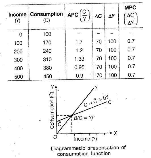
Complete the Core Trio (Y, C, S): Use the formula $Y = C + S$ to find the missing one. For example, if Y and C are given, the first thing you should do is calculate a column for S.
Calculate the 'Change' Columns ( $Δ$ ): To find MPC or MPS, you need the change between levels. Calculate $Δ Y$ , $Δ C$ , and $Δ S$ . For example, $Δ Y$ at the second level of income is $Y_{2} - Y_{1}$ .
Calculate the Propensities: Use the appropriate formulas ( $C / Y$ , $Δ C /Δ Y$ , etc.) to fill in the APC, APS, MPC, or MPS columns.
Work Backwards if Needed: Sometimes, you'll be given a propensity (like a constant MPC) and need to find C or S. This is where you reverse the logic. For example, if you know $Δ Y$ and MPC, you can find $Δ C$ using the formula $Δ C = M P C \times Δ Y$ . You can then find the next level of consumption by adding this $Δ C$ to the previous level of consumption.

Let's see this strategy in action.

3. Guided Example 1: The Standard Case

In the most common type of problem, you are given Income (Y) and Consumption (C) and asked to find the rest. The following video provides an excellent walkthrough.

Determination of income & employment Numericals The end. AD- AS Part 10 Most important Numericals

This video by Sunil Panda demonstrates how to complete a table when income and consumption schedules are given.

Watch the instructor solve the problem from this table. Observe the step-by-step process: He calculates APC (C/Y) first. He then uses the relationship APC + APS = 1 to find APS without even needing to calculate Savings first. This is a smart shortcut. To find MPC, he first calculates \Delta C and \Delta Y. Finally, he uses MPC to find the multiplier (K), linking back to our previous lesson.

4. Guided Example 2: Working Backwards

Now, let's tackle a slightly more complex problem where you have to work backwards from the given information. In this case, you are given Income (Y), a constant MPC, and one value for Savings.

Determination of income & employment Numericals The end. AD- AS Part 10 Most important Numericals

This next segment from the same video shows how to solve a problem where you must use the given propensities to derive the core values.

Watch the solution from this problem. Pay close attention to the logic: Find \Delta Y: He starts by calculating the change in income, which is constant. Use MPC to find \Delta C: Since MPC and \Delta Y are known, he calculates \Delta C = MPC \times \Delta Y. This gives him a constant change in consumption. Find Autonomous Consumption (\bar{C}): He uses the initial saving value (-30) at zero income to deduce that autonomous consumption must be +30. This is a key step. Complete the C column: Starting with autonomous consumption (30), he repeatedly adds the calculated \Delta C (75) to find all the consumption values. Complete the remaining columns (S, APC, etc.): Once Y and C are known, the rest is straightforward.

This backward method is a very important skill, as it tests a deeper understanding of the relationships.

5. Your Turn: Practice with Exam-Style Questions

Now it's time for you to apply these methods. Solving these yourself is the best way to prepare.

First, let's practice with a few standard problems. The resource below provides clear, solved examples.

[Macroecomics] Practical Questions - MPC and MPS - Teachoo

This resource from Teachoo provides several well-explained examples of table-completion problems, typical of what you might see in your exam.

In your notebook, solve Example 7 and Example 8. In Example 7, you are given Y and C. In Example 8, you are given Y and S. First, try to solve them completely on your own, creating the full table with all the required columns. Then, click "View Answer" on the webpage to check your work and the methodology.

Excellent. Now for a direct challenge from a past paper. Solve the question in the image below in your notebook.

This is a typical board exam question. You are given Income (Y) and Consumption (C) at different levels. You need to calculate Savings (S), Average Propensity to Consume (APC), and Marginal Propensity to Save (MPS). You are also asked for the consumption function.

Solution Check:
After you have completed the table, check your answers below.

Savings (S): -40, 0, 40
Average Propensity to Consume (APC): -, 1.0, 0.93
Marginal Propensity to Save (MPS): -, 0.4, 0.4
Consumption Function: At Y=200, C is 120. We can see $Δ C = 40$ and $Δ Y = 50$ , so MPC (b) = $Δ C /Δ Y = 40/50 = 0.8$ . Autonomous consumption ( $C ˉ$ ) is 40 (C when Y=0). Therefore, the consumption function is $C = 40 + 0.8 Y$ .

Conclusion

In this lesson, we transitioned from using formulas in isolation to applying them within the structure of an income-consumption-saving schedule. This practical skill is vital for scoring well on the numerical questions in your exam.

Key Takeaways:

All table-based problems are solved using the seven fundamental relationships between Y, C, S, and their propensities.
The strategy is to work systematically: use $Y = C + S$ to find the core values, then calculate the changes ( $Δ$ ), and finally derive the propensities.
Be prepared to work backwards: use a given MPC or MPS to calculate $Δ C$ or $Δ S$ , and then build up the consumption or saving schedules.

You are now well-equipped to handle this type of question. In our next session, we will continue our numerical focus by tackling categorized board paper questions that specifically test your understanding of propensities (APC, MPC, etc.). This will help you build even more speed and confidence for the exam.