Calculating Equilibrium: Income, Consumption, and Savings

Hello! In our last lesson, we focused on the building blocks of consumption and saving behavior by calculating the various propensities (APC, APS, MPC, and MPS). We saw how these ratios describe spending patterns from both total and additional income.

Now, we will use that foundation, particularly the consumption function and MPC, to tackle one of the most important numerical problems in macroeconomics. This lesson will show you how to algebraically determine the equilibrium point of an economy—the level of income where aggregate demand equals aggregate supply. Mastering this is crucial for your board exams, as these questions are very common.

Today's learning outcome is to: Solve for equilibrium income, consumption, and savings given the consumption/saving function and investment.

1. The Two Conditions for Equilibrium

In the theoretical lessons, you learned that in a simple two-sector economy (households and firms), equilibrium is achieved when one of two conditions is met. For numerical problems, we translate these conditions into solvable equations:

Aggregate Demand (AD) = Aggregate Supply (AS)
- We know that AS is simply the national income (Y).
- AD is the sum of Consumption (C) and Investment (I).
- Therefore, the equilibrium equation is: $Y = C + I$
Savings (S) = Investment (I)
- This condition states that the part of income that is not spent (leakages) must equal the amount injected back into the economy as investment.
- The equilibrium equation is: $S = I$

Both approaches will always give you the same equilibrium level of income. The AD = AS approach is more direct, while the S = I approach can sometimes be faster if you are given the saving function directly.

2. Solving for Equilibrium: The AD = AS Approach

This is the most common method. The goal is to find the value of Income (Y) that makes the equation $Y = C + I$ true.

The process is straightforward algebra:

Start with the equilibrium condition: $Y = C + I$
Substitute the consumption function, $C = C ˉ + bY$ , into the equation. ( $C ˉ$ is Autonomous Consumption, and $b$ is MPC).
The equation becomes: $Y = (C ˉ + bY) + I$
Group all terms with Y on one side: $Y - bY = C ˉ + I$
Factor out Y: $Y (1 - b) = C ˉ + I$
Solve for Y: $Y = \frac{C ˉ + I}{1 - b}$

The following video provides an excellent step-by-step demonstration of this method to solve for equilibrium income, consumption, and savings.

Important Numericals | 12th Commerce | Determination Of Income & Employment🔥

This video from Commerce Wallah by PW clearly explains the fundamental formulas and then walks through two detailed examples of calculating equilibrium income (Y), consumption (C), and savings (S).

First, watch the Formulas review. This will quickly refresh the key equations for AD, AS, C, S, and the equilibrium conditions. Next, follow the first solved example. The instructor calculates equilibrium Y, then uses it to find C and S. This is the core procedure you need to master. Finally, watch the second solved example for reinforcement. Seeing the process repeated with different numbers will solidify your understanding.

As you saw in the video, once you calculate the equilibrium income (Y), finding the other two values is simple:

Equilibrium Consumption (C): Substitute the value of Y back into the given consumption function.
Equilibrium Savings (S): Either use the formula $S = Y - C$ , or substitute Y into the saving function if you have it.

3. The Alternative: Solving with the S = I Approach

The second equilibrium condition, $S = I$ , provides an alternative, often quicker, route to the same answer.

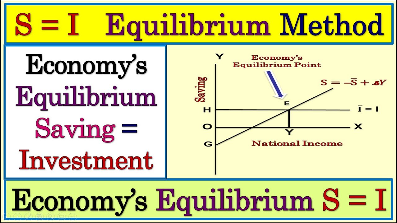
This graph illustrates the S=I equilibrium method. The economy is in equilibrium at point E, where the amount households plan to save is exactly equal to the amount firms plan to invest. Our goal is to find the income level (Y) where this occurs.

To use this method algebraically:

Start with the equilibrium condition: $S = I$
Recall the saving function is $S = - C ˉ + (1 - b) Y$ , where $(1 - b)$ is the MPS.
The equation becomes: $- C ˉ + (1 - b) Y = I$
Rearrange to solve for Y: $(1 - b) Y = C ˉ + I$
Solve for Y: $Y = \frac{C ˉ + I}{1 - b}$

Notice this is the exact same final formula as the AD=AS method. This is a great way to check your work if you have time.

4. Practice with Past Board Questions

Your goal is to solve these problems quickly and accurately under exam pressure. Let's work through some variations from past papers.

Guided Practice: Calculating Equilibrium Values

This is the most common type of question. You are given the consumption function and investment and asked to find equilibrium Y, C, or S.

Most Important PYQs | Macro Economics | Chapter 7,8,9

In this clip from his "Most Important PYQs" series, Rajat Arora solves a typical board question.

Watch the segment from this equilibrium problem. He calculates equilibrium income (Y), aggregate demand (AD) at equilibrium, and the Marginal Propensity to Save (MPS). Notice how he confirms that at equilibrium, Y = AD.

Guided Practice: Checking for Equilibrium

Sometimes, a question will give you an income level and ask if the economy is in equilibrium. In this case, you don't solve for Y. Instead, you plug the given Y into the AD formula ( $C + I$ ) and see if the result equals Y.

Most Important PYQs | Macro Economics | Chapter 7,8,9

Let's watch another problem from the same video. Here, the task is to determine if the economy is in equilibrium at a given income level.

Watch the explanation from the first question. The instructor calculates AD at the given income level of 2000 and compares it to AS (which is 2000). Since they are not equal, the economy is not in equilibrium.

5. Your Turn: Solving CBSE Numericals

Now it's time for you to practice. The following resource is a collection of solved questions from past CBSE exams. Your task is to solve them on your own first, then check your method against the solution.

NCERT Solutions for Class 12 Macro Economics National Income ...

This webpage contains a list of numerical problems, many taken directly from past CBSE papers. This is excellent practice for your exam.

Find and solve the following questions on the page: Question 8: Given C = 200 + 0.75Y and I = 4000. Calculate equilibrium Y and C. Question 11: Given C = 100 + 0.75Y and I = 1000. Calculate equilibrium Y and C. Question 14: Given Autonomous C = 100, MPC = 0.80, and I = 50. Calculate National Income (Y). First, solve these using the Y = C + I method in your notebook. Then, compare your answers and steps to the solutions provided in the resource.

For reference, here is an example of how a fully solved answer might be presented in an exam. Note the clear statement of the equilibrium condition and the step-by-step algebra.

This image shows well-structured solutions for past CBSE paper questions. This is a good format to follow for your own answers.

Conclusion

In this lesson, we bridged the gap between theory and numerical application. You learned how to take the equilibrium conditions and use them to find the exact point where an economy's income, spending, and saving are in balance.

Key Takeaways:

Equilibrium in a two-sector economy occurs when $Y = C + I$ or, alternatively, when $S = I$ .
To solve for equilibrium income (Y), substitute the given consumption function and investment value into the equilibrium equation and solve for Y.
Once you have equilibrium Y, you can find equilibrium C by plugging Y back into the consumption function, and equilibrium S by using $S = Y - C$ .
Practice with past paper questions is the key to building the speed and confidence needed for your board exam.

In our next lesson, we will explore one of the most powerful concepts in this chapter: the investment multiplier. You'll learn to calculate its value and see how a change in investment can lead to a much larger change in national income. The formula for the multiplier is derived directly from the equilibrium equation we mastered today.

Recommended resources