Hello! Let's get started with today's lesson.
Introduction
In our last lesson, we focused on the theory behind L1 (LASSO) and L2 (Ridge) regularization. We established that:
- Ridge (L2) adds a penalty based on the squared coefficients, which shrinks them towards zero.
- LASSO (L1) adds a penalty based on the absolute value of coefficients, which not only shrinks them but can force some to become exactly zero.
Today, we'll move from theory to practice. Our goal is to apply both Ridge and Lasso regression using scikit-learn. You will see firsthand how these models affect the coefficients and how LASSO's unique property serves as a form of automatic feature selection.
Applying LASSO and Observing Coefficients
Let's dive straight into the code. The process of applying a regularized model follows the standard machine learning workflow you're familiar with: load data, split, scale, train, and evaluate.
Scaling is particularly important for regularized models. Since the penalty is based on the magnitude of the coefficients, features with different scales can be penalized unfairly. StandardScaler ensures all features are on a level playing field.
The following video provides a clear, step-by-step implementation of LASSO regression on the California Housing dataset.
Lasso Regression with Scikit-Learn (Beginner Friendly)
This video, 'Lasso Regression with Scikit-Learn', walks through the entire process, from data preparation to fitting the model and inspecting the results. It's a great example of a typical workflow.
Please watch from 01:10 to 16:01. Focus on these key stages: Data Prep (01:10 - 06:25): Observe the standard use of train_test_split and StandardScaler. Fitting the Model (06:25 - 08:46): See how Lasso is imported and fit to the training data. Hyperparameter Tuning (08:46 - 11:40): Pay attention to how GridSearchCV is used to find a good value for the regularization strength, alpha. Inspecting Coefficients (11:40 - 16:01): This is the most important part. Notice how the final coefficients are extracted and displayed in a Pandas DataFrame. Identify which features have coefficients that are zero or very close to it.
As you saw, the implementation is straightforward. The most revealing part is when the coefficients are paired with their feature names in a DataFrame. With an appropriate alpha, LASSO effectively "turned off" some features by setting their coefficients to zero, simplifying the model.
Applying Ridge and Comparing Results
The process for applying Ridge regression is nearly identical. You import Ridge from sklearn.linear_model, instantiate it with an alpha, and fit it to your scaled training data.
from sklearn.linear_model import Ridge


# The workflow is the same:
# 1. Instantiate the model with a chosen alpha
ridge_model = Ridge(alpha=1.0)


# 2. Fit on scaled training data
ridge_model.fit(X_train_scaled, y_train)


# 3. Inspect the coefficients
print(ridge_model.coef_)
The crucial difference isn't in the code workflow, but in the output. Where LASSO might produce a list of coefficients like [0, 520.8, 291.1, -90.0, 0, ...], Ridge would produce something like [-3.6, 511.2, 313.5, -161.5, -19.8, ...].
Notice that all coefficients in the Ridge example are non-zero. They have been "shrunk" compared to a standard linear regression, but no feature has been completely removed.
To see a direct, side-by-side comparison, let's examine a summary table from the article "Building and Regularizing Linear Regression Models". It shows the coefficients from an unregularized linear model, a Ridge model, and a LASSO model, all trained on the same dataset.
Building and Regularizing Linear Regression Models in Scikit-learn
This article provides an excellent summary table that contrasts the coefficient values from three different models.
Please read the short 'Summary' section. Focus on the DataFrame and the plot that compare the coefficients from 'without_regularization', 'Ridge', and 'Lasso'.
The table from the article is a perfect illustration of what we've discussed.
| without_regularization | Ridge | Lasso | |
|---|---|---|---|
| age | -10.0122 | -3.60965 | -0 |
| sex | -239.819 | -224.329 | -186.309 |
| bmi | 519.84 | 511.204 | 520.894 |
| bp | 324.39 | 313.553 | 291.196 |
| s1 | -792.184 | -161.534 | -90.0686 |
| s2 | 476.746 | -19.893 | -0 |
| s3 | 101.045 | -166.68 | -220.207 |
| s4 | 177.064 | 113.95 | 0 |
| s5 | 751.279 | 496.222 | 506.422 |
| s6 | 67.6254 | 77.4439 | 49.0746 |
As highlighted, LASSO drove the coefficients for 'age', 's2', and 's4' to exactly zero, effectively performing feature selection. Ridge, in contrast, retained all features but reduced the magnitude of their coefficients.
Visualizing the Regularization Path
A powerful way to visualize the effect of the regularization strength alpha is by plotting the "regularization path." This plot shows how the value of each coefficient changes as alpha increases.
LASSO Path
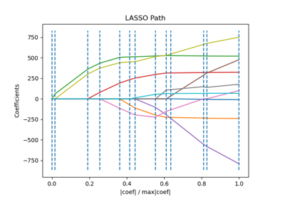
In the LASSO path, you can clearly see lines (coefficients) collapsing to the zero-axis. This is the visual signature of LASSO's feature selection capability.
Ridge Path
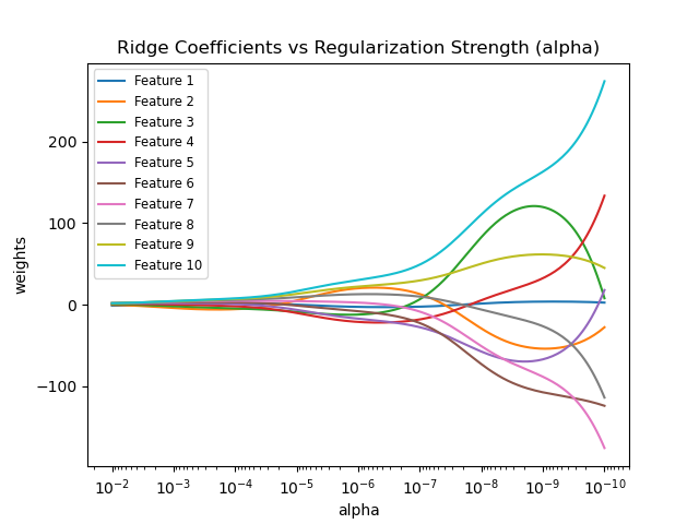
The Ridge path looks quite different. The coefficients are all pulled towards zero as alpha increases, but they don't hit the zero line. All features remain in the model, just with diminished influence.
Conclusion
In this lesson, we put theory into practice. You've now seen how to implement and interpret Ridge and LASSO regression models in scikit-learn.
Key Takeaways:
- Both
RidgeandLassoare implemented in scikit-learn with a similar workflow, controlled by thealphahyperparameter. - Feature scaling (e.g., using
StandardScaler) is a critical preprocessing step for these models. - LASSO (L1) can shrink coefficients to exactly zero, making it a valuable tool for automatic feature selection and creating simpler, more interpretable models.
- Ridge (L2) shrinks all coefficients towards zero but does not eliminate them. It is effective at reducing model complexity and handling multicollinearity when you believe all features are relevant.
- The effect of each model on the coefficients is clearly visible when you inspect the final coefficient values or visualize the regularization path.
Preview of the Next Lesson
In the video, you saw GridSearchCV used to find the best alpha. While we've focused on the effect of alpha today, our next lesson will be dedicated to the method of finding its optimal value. We will take a deeper dive into cross-validation as a robust strategy for hyperparameter tuning.