Sigmoid Function in Logistic Regression

From Linear to Logistic: The Need for Probabilities

You've already encountered linear regression in your studies, which models a relationship like $y={\mathbf{w}}^T\mathbf{x}+b$ to predict a continuous value. A natural first thought for a binary classification problem (e.g., predicting if a customer will buy insurance: yes/no, 1/0) might be to try and fit a straight line to the data.

However, this approach has two major flaws:

1. Unbounded Output: A linear model's output can be any number, from $-\infty$ to $+\infty$. This doesn't make sense for classification, where we want a probability between 0 and 1. How would you interpret a prediction of 1.5 or -0.2?
2. Sensitivity to Outliers: The line of best fit can be heavily skewed by new data points, especially outliers. This can cause the decision threshold (e.g., classifying anything above 0.5 as "1") to shift, leading to incorrect classifications for existing points.

Let's watch a couple of short video clips that illustrate these problems perfectly.

The Solution: The Sigmoid Function

To solve this, we need a way to take the unbounded output of the linear equation ($z={\mathbf{w}}^T\mathbf{x}+b$) and "squash" it into a valid probability range of [0, 1]. This is exactly what the sigmoid function does.

The sigmoid function, sometimes called the logistic function, is defined as:
$\sigma (z)=\frac{1}{1+e^{-z}}$

It produces a characteristic "S-shaped" curve.

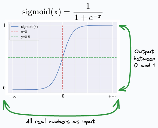
No matter how large or small the input $z$ is, the output $\sigma (z)$ will always be between 0 and 1.

• As $z$ approaches $+\infty$, $e^{-z}$ approaches 0, so $\sigma (z)$ approaches $\frac{1}{1+0}=1$.
• As $z$ approaches $-\infty$, $e^{-z}$ approaches $+\infty$, so $\sigma (z)$ approaches 0.
• When $z=0$, $\sigma (z)=\frac{1}{1+e^0}=\frac{1}{2}=0.5$.

This elegant mathematical trick allows us to interpret the output directly as a probability. For example, if our model outputs 0.93, we can say there is a 93% probability that the sample belongs to the positive class (class 1).

The following reading from Google's Machine Learning Crash Course provides an excellent and concise explanation of this core concept.

Check Your Understanding

Let's quickly test this idea. Based on the article you just read, consider a logistic regression model with the following weights:

• Bias: $b=1$
• Weight 1: $w_1=2$
• Weight 2: $w_2=-1$
• Weight 3: $w_3=5$

And an input example with these feature values:

• Feature 1: $x_1=0$
• Feature 2: $x_2=10$
• Feature 3: $x_3=2$

1. First, calculate the linear output, $z$:
$z=b+w_1{x}_1+w_2{x}_2+w_3{x}_3$

2. Now, plug this value of $z$ into the sigmoid function to get the final probability:
$P(y=1)=\sigma (z)=\frac{1}{1+e^{-z}}$
(You can use a calculator. $e^{-1}\approx 0.367$)

This two-step process—calculating a linear score $z$ and then passing it through the sigmoid function—is the heart of logistic regression.

Conclusion

In this lesson, we bridged the gap between linear models and classification by introducing the sigmoid function. You saw why linear regression is a poor choice for classification tasks and how logistic regression elegantly solves the problem.

Key Takeaways:

• Logistic regression, despite its name, is a classification algorithm.
• It cannot use a linear model's output directly because the output is unbounded and not a valid probability.
• The core of logistic regression is the sigmoid function, $\sigma (z)=1/(1+e^{-z})$, which squashes any real number into the range (0, 1).
• The final output is interpreted as the probability of the sample belonging to the positive class (e.g., class "1").

Preview of the Next Lesson

We now understand what a logistic regression model predicts and how it formulates that prediction as a probability. But how does the model learn the best values for its weights ($w$) and bias ($b$)? In the next lesson, we will explore the loss function used to train logistic regression, which is known as cross-entropy loss. This will give us the complete picture of how the model is trained from data.