Calculating Structure Functions in the Naive Parton Model

1. The Naive Parton Model

The naive parton model, proposed by Feynman, rests on a simple but powerful physical picture. In a reference frame where the proton is moving with nearly the speed of light (the "infinite momentum frame"), its internal dynamics are slowed down by time dilation. From the perspective of the incoming high-energy electron, the proton's constituents (partons) are effectively "frozen" and non-interacting for the brief duration of the collision.

The core assumptions are:

1. The proton is a collection of point-like constituents (partons).
2. In the infinite momentum frame, these partons are effectively free and do not interact with each other during the scattering event.
3. The scattering of the electron from the proton is an incoherent sum of elastic scattering events between the electron and each individual parton.

This allows us to write the overall cross-section for electron-proton scattering as a sum over the cross-sections for electron-parton scattering, weighted by the probability of finding a given parton inside the proton.

The central idea is captured in the formula:
$d\sigma (ep\to eX)={\sum }_i{\int }_0^{1}d\xi f_i(\xi )d\hat{\sigma }(e+{\text{parton}}_i(\xi p)\to e+{\text{parton}}_i)$
Here:

• $\xi$ is the fraction of the proton's momentum carried by the parton.
• $f_i(\xi )$ is the Parton Distribution Function (PDF) for a parton of type $i$. It represents the probability density to find parton $i$ inside the proton carrying momentum fraction $\xi$.
• $d\hat{\sigma }$ is the cross-section for the fundamental (partonic) elastic scattering process. The 'hat' denotes a partonic-level quantity.

The PDFs, $f_i(\xi )$, are non-perturbative quantities. They cannot be calculated from first principles within perturbation theory but must be determined from experiment. However, QCD predicts how they evolve with the energy scale $Q^2$, and crucially, they are universal—a PDF measured in electron-proton scattering can be used to predict the outcome of proton-proton collisions at the LHC.

2. The Inhabitants of the Proton

So, what are these partons? The simplest idea would be to identify them with the three "valence" quarks of the Gell-Mann quark model (uud for the proton). However, reality is more complex.

As the video explains, the proton is a dynamic, quantum-mechanical system. Its constituents are:

• Valence Quarks: The two up quarks and one down quark ($u_v,u_v,d_v$) that determine the proton's overall quantum numbers (charge +1, baryon number 1).
• Sea Quarks: A fluctuating "sea" of quark-antiquark pairs ($u\bar{u},d\bar{d},s\bar{s},\dots$) created by gluons splitting.
• Gluons: The gauge bosons of the strong force that bind the quarks together. While they don't interact with the virtual photon directly (they have no electric charge), they carry a significant fraction of the proton's momentum.

The PDFs for a proton, $f_i(x)$, are often written as $u(x),d(x),s(x),\bar{u}(x),\bar{d}(x),\bar{s}(x)$, etc., and $g(x)$ for the gluon. For example, $u(x)=u_v(x)+u_{sea}(x)$.

A key experimental finding is the momentum sum rule. The total momentum of the proton is the sum of the momenta of its constituents:
${\sum }_i{\int }_0^{1}dxx{f}_i(x)={\int }_0^{1}dxx\left[{\sum }_q(q(x)+\bar{q}(x))+g(x)\right]=1$
Experimentally, it's found that the quarks and antiquarks together carry only about 50% of the proton's total momentum. This was compelling indirect evidence for gluons, which must carry the remaining ~50%.

3. Calculating the Structure Functions

Now we have all the pieces to calculate the structure functions. We will relate the hadronic tensor $W^{\mu \nu }$ (which defines $F_1$ and $F_2$) to the partonic tensor ${\hat{w}}^{\mu \nu }$ using the master formula of the parton model.

Recall from the previous lesson the general decomposition of the hadronic tensor:
$W^{\mu \nu }=\left(-g^{\mu \nu }+\frac{q^{\mu }{q}^{\nu }}{q^2}\right)W_1+\frac{1}{M_p^2}\left(p^{\mu }-\frac{p\cdot q}{q^2}{q}^{\mu }\right)\left(p^{\nu }-\frac{p\cdot q}{q^2}{q}^{\nu }\right)W_2$
In the parton model, this becomes:
$W^{\mu \nu }(p,q)={\sum }_i{\int }_0^{1}d\xi f_i(\xi ){\hat{w}}_i^{\mu \nu }(\xi p,q)$
Our task is to calculate the partonic tensor ${\hat{w}}_i^{\mu \nu }$ for elastic scattering of an electron off a spin-1/2 quark of charge $e_i$. This is a QED calculation very similar to those you've seen for electron-muon scattering.

Let's summarize the key results of that derivation.

1. Kinematic Constraint: The on-shell condition for the scattered quark with initial momentum $\xi p$ is $(\xi p+q{)}^2=m_q^2\approx 0$. Expanding this gives ${\xi }^2{p}^2+2\xi p\cdot q+q^2\approx 0$. In the high-energy limit where the proton mass can be neglected ($p^2=M_p^2\approx 0$), this simplifies to $2\xi p\cdot q-Q^2=0$, or:
   $\xi =\frac{Q^2}{2p\cdot q}=x$
   This is a remarkable result. It shows that the momentum fraction $\xi$ of the struck parton is identically equal to the experimentally measurable Bjorken variable $x$.

2. Partonic Tensor Calculation: The calculation yields the partonic tensor ${\hat{w}}_i^{\mu \nu }$, which contains the kinematic constraint $\delta (\xi -x)$.

3. Hadronic Structure Functions: By substituting the calculated ${\hat{w}}^{\mu \nu }$ back into the integral for $W^{\mu \nu }$ and comparing the result to the general definition of $W_1$ and $W_2$ (or equivalently $F_1$ and $F_2$), we can extract their form in the parton model. The integration over $\xi$ is trivial due to the $\delta (\xi -x)$.

The final result for the structure function $F_2$ is:
$F_2(x)={\sum }_i{e}_i^{2}x{f}_i(x)$
Here, the sum is over all quark and antiquark flavors $i=u,d,s,\bar{u},\bar{d},\bar{s},\dots$, and $e_i$ is the electric charge of quark $i$ in units of $e$ (e.g., $e_u=+2/3$, $e_d=-1/3$).

4. Interpretation and Physical Meaning

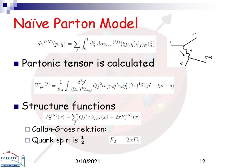
The formula $F_2(x)={\sum }_i{e}_i^{2}x{f}_i(x)$ is the central achievement of the naive parton model. It accomplishes several things:

• It gives a physical meaning to $F_2(x)$: This experimentally measurable function is now understood as the charge-squared-weighted sum of the momentum distributions of the quarks in the proton.
• It explains Bjorken scaling: In this naive model, the PDFs $f_i(x)$ and therefore $F_2(x)$ depend only on $x$, not on $Q^2$. This provides a direct theoretical explanation for the scaling behavior observed at SLAC. (In full QCD, there are logarithmic corrections to this scaling, which we will discuss later).
• It becomes a predictive tool: If we measure $F_2$ in electron-proton scattering, we can extract information about the PDFs. We can then use these PDFs to predict the outcomes of other processes, like neutrino-proton scattering or proton-proton collisions.

Conclusion

Key Takeaways:

• The naive parton model successfully describes DIS by treating it as an incoherent sum of elastic scatters off quasi-free, point-like partons (quarks) inside the proton.
• The model introduces Parton Distribution Functions (PDFs), $f_i(x)$, which describe the probability of finding a parton of type $i$ with momentum fraction $x$.
• A direct calculation based on QED for the electron-quark interaction allows us to predict the form of the proton's structure function $F_2(x)$.
• The result, $F_2(x)={\sum }_i{e}_i^{2}x{f}_i(x)$, provides a profound physical interpretation for $F_2$ and explains the phenomenon of Bjorken scaling.

You have now connected a macroscopic, experimental observable ($F_2$) to the microscopic, fundamental constituents of matter (quarks and their charges). This is a cornerstone of our understanding of hadronic physics and the Standard Model.

Preview of the Next Lesson:

In our calculation of the hadronic tensor, we focused on extracting $F_2$. However, the calculation also yields a prediction for the other structure function, $F_1$. In the next lesson, we will derive the Callan-Gross relation, a specific relationship between $F_1$ and $F_2$ that emerges directly from this model, and explain how its experimental verification provided definitive evidence that the partons have spin-1/2.