Neutrino-Electron Scattering: Z Boson Mediated Cross-Section

Hello! Welcome back to our journey through electroweak phenomenology.

In the last lesson, you successfully calculated the decay rate of the W boson, a process governed by the charged current. You saw how to apply Feynman rules, use trace technology for a 1→2 decay, and connect the theoretical Lagrangian to a measurable quantity, the decay width.

Today, we shift our focus from decays to scattering, and from the charged current to the neutral current. We will tackle another cornerstone process of the Standard Model. By the end of this lesson, you will be able to:

Calculate the tree-level cross-section for neutrino-electron scattering mediated by the Z boson.

This will involve a 2→2 scattering process, a natural step up in complexity from the 1→2 decay we studied previously. We'll specifically analyze the reaction $ν_{μ} + e^{-} \to ν_{μ} + e^{-}$ . We choose the muon neutrino because this reaction proceeds only through the exchange of a $Z$ boson at tree level. This isolates the neutral current interaction cleanly, providing a perfect testbed for our theoretical tools.

1. The Neutral Current Vertex

Our starting point is the neutral current interaction Lagrangian, which we derived previously. This part of the electroweak Lagrangian describes how the $Z$ boson couples to fermions:

L_{N C} = - \frac{g}{cos θ _{W}} Z_{μ} J_{N C}^{μ}

where the neutral current $J_{N C}^{μ}$ for a fermion $f$ is given by:

J_{N C}^{μ} = f ˉ γ^{μ} \frac{1}{2} (c_{V}^{f} - c_{A}^{f} γ^{5}) f

The crucial components here are the vector coupling $c_{V}^{f}$ and the axial-vector coupling $c_{A}^{f}$ . These constants depend on the fermion's weak isospin ( $T^{3}$ ) and electric charge ( $Q$ ).

Chapter 11 Electroweak interactions

To derive the Feynman rule for the Z-fermion vertex and understand where these couplings come from, let's review a key section from the 'Electroweak interactions' chapter we've touched on before.

Please read section 11.7 'Electroweak Feynman rules', focusing on the derivation of the neutral current vertex ('iLNC_int'). Pay close attention to the definitions of the couplings c_V and c_A in equations (11.19) and (11.20), and look at Table 11.3, which lists their values for different fermions.

From the reading, the Feynman rule for a $Z$ -fermion-fermion vertex is:

Vertex = - i \frac{g}{cos θ _{W}} γ^{μ} \frac{1}{2} (c_{V}^{f} - c_{A}^{f} γ^{5})

Using Table 11.3 from the resource (and your knowledge of weak isospin and hypercharge), we can find the specific couplings for our particles:

For the electron ( $e^{-}$ ): $Q_{e} = - 1$ , $T_{L}^{3} = - 1/2$ .
- $c_{V}^{e} = T^{3} - 2 sin^{2} θ_{W} Q_{e} = - 1/2 + 2 sin^{2} θ_{W}$
- $c_{A}^{e} = T^{3} = - 1/2$
For the muon neutrino ( $ν_{μ}$ ): $Q_{ν} = 0$ , $T_{L}^{3} = + 1/2$ .
- $c_{V}^{ν} = T^{3} - 2 sin^{2} θ_{W} Q_{ν} = 1/2$
- $c_{A}^{ν} = T^{3} = 1/2$

Notice that for the neutrino, $c_{V}^{ν} = c_{A}^{ν} = 1/2$ , so the vertex term becomes $γ^{μ} (1/2 - 1/2 γ^{5}) = γ^{μ} P_{L}$ . This confirms that only left-handed neutrinos participate in the weak interaction, as expected.

2. The Scattering Process and Matrix Element

We are now ready to analyze the scattering process $ν_{μ} (p_{1}) + e^{-} (p_{2}) \to ν_{μ} (p_{3}) + e^{-} (p_{4})$ .

Neutrino-Electron Scattering Diagrams and Cross-Sections — This figure displays the Feynman diagram for elastic neutrino-electron scattering mediated by a Z boson. The incoming neutrino and electron exchange a Z boson, resulting in their scattering. The diagram on the right shows the low-energy approximation, where the interaction can be treated as a point-like four-fermion vertex.

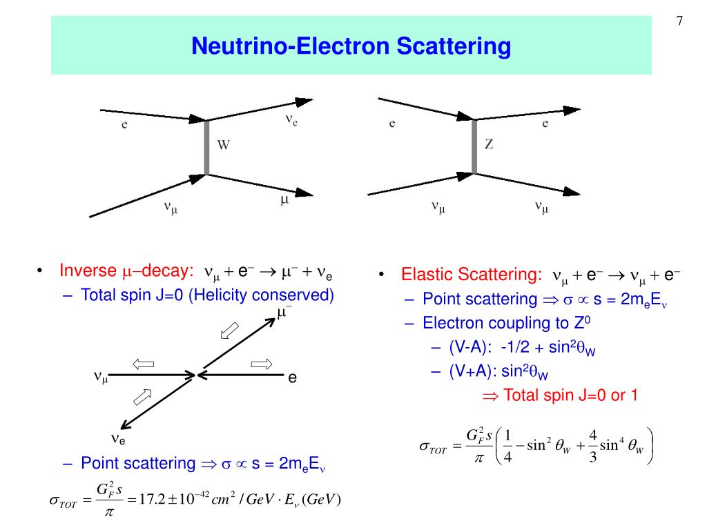
This is a t-channel process where the four-momentum carried by the $Z$ boson is $q = p_{1} - p_{3} = p_{4} - p_{2}$ .

The invariant matrix element $M$ is constructed by combining two vertices with the Z boson propagator:

i M = [u ˉ (p_{3}) (- i \frac{g}{2 cos θ _{W}}) γ^{μ} (c_{V}^{ν} - c_{A}^{ν} γ^{5}) u (p_{1})] \times [\frac{- i ( g _{μν} - q _{μ} q _{ν} / M _{Z}^{2} )}{q ^{2} - M _{Z}^{2}}] \times [u ˉ (p_{4}) (- i \frac{g}{2 cos θ _{W}}) γ^{ν} (c_{V}^{e} - c_{A}^{e} γ^{5}) u (p_{2})]

The Low-Energy Approximation

For many practical scenarios (like neutrinos from nuclear reactors or accelerators), the momentum transfer is small compared to the Z boson mass ( $q^{2} ≪ M_{Z}^{2} \approx (91 GeV)^{2}$ ). In this limit:

The propagator denominator simplifies: $q^{2} - M_{Z}^{2} \approx - M_{Z}^{2}$ .
The $q_{μ} q_{ν} / M_{Z}^{2}$ term in the numerator can be neglected. (This term would contract with the fermion currents, and its contribution is suppressed by factors of $m_{f} / M_{Z}$ , making it negligible for light fermions).

The propagator thus becomes $\approx \frac{i g _{μν}}{M _{Z}^{2}}$ . The matrix element simplifies to:

i M \approx - i (\frac{g ^{2}}{4 cos ^{2} θ _{W} M _{Z}^{2}}) [u ˉ_{3} γ^{μ} (c_{V}^{ν} - c_{A}^{ν} γ^{5}) u_{1}] [u ˉ_{4} γ_{μ} (c_{V}^{e} - c_{A}^{e} γ^{5}) u_{2}]

Using the relations $g = e / sin θ_{W}$ and $M_{W} = M_{Z} cos θ_{W}$ , along with $\frac{G _{F}}{2} = \frac{g ^{2}}{8 M _{W}^{2}}$ , we can rewrite the prefactor:

\frac{g ^{2}}{4 cos ^{2} θ _{W} M _{Z}^{2}} = \frac{g ^{2}}{4 M _{W}^{2}} = 2 \frac{g ^{2}}{8 M _{W}^{2}} = 2 \frac{G _{F}}{2} = 2 G_{F}

So, the matrix element becomes that of an effective four-fermion interaction:

M = \frac{G _{F}}{2} [u ˉ_{3} γ^{μ} (1 - γ^{5}) u_{1}] [u ˉ_{4} γ_{μ} (c_{V}^{e} - c_{A}^{e} γ^{5}) u_{2}]

We've substituted $c_{V}^{ν} = c_{A}^{ν} = 1/2$ , giving the $(1 - γ^{5})$ factor for the neutrino current.

3. Calculating the Cross-Section

The next step is to calculate the unpolarized squared matrix element, $⟨ ∣ M ∣^{2} ⟩$ . We average over the two initial electron spins and sum over all final state spins. (The incoming neutrino is always left-handed, so no averaging is needed for it).

⟨ ∣ M ∣^{2} ⟩ = \frac{1}{2} spins \sum ∣ M ∣^{2}

This calculation involves standard trace technology, similar to what you did for the W decay. The result is a product of two traces, one for the neutrino line and one for the electron line. The algebra is lengthy, so we'll utilize a resource that presents the result in a clean and standard form.

The differential cross-section is often expressed in terms of the lab-frame inelasticity, $y$ , defined as the fraction of the incoming neutrino's energy transferred to the electron's kinetic energy.

From eV to EeV: Neutrino Cross-Sections Across Energy...

The following paper provides a concise summary of the formalism for neutrino-lepton scattering and gives the final formulas for the differential cross-section.

Please start by reading the first part of section B, 'Formalism: Matrix Elements' to see the general structure of the neutral current. Then, jump to the formulas for the differential cross-sections dσ/dy near the end of the section (after Eq. 19). Note how the paper defines its own gV and gA, which combine the couplings from the neutrino and electron lines. Finally, look at Table I, which provides the values for the left- and right-handed couplings for all fermions.

The resource gives the differential cross-section for $ν_{l} e \to ν_{l} e$ scattering as:

\frac{d σ}{d y} = \frac{G _{F}^{2} m _{e} E _{ν}}{2 π} [(g_{V} + g_{A})^{2} + (g_{V} - g_{A})^{2} (1 - y)^{2} - (g_{V}^{2} - g_{A}^{2}) \frac{m _{e} y}{E _{ν}}]

where $E_{ν}$ is the lab-frame neutrino energy and the electron is assumed to be at rest initially. The term $(g_{V}^{2} - g_{A}^{2}) \frac{m _{e} y}{E _{ν}}$ is very small for high-energy neutrinos and can often be neglected.

The couplings $g_{V}$ and $g_{A}$ in this formula are effective combinations for the whole process. Comparing our matrix element with the one in the paper (Eq. 18), we can match the terms. The paper's couplings are related to our fundamental $c_{V}, c_{A}$ values as follows (using the notation from Table I in the resource):

$g_{V} = 2 g_{L}^{ν} g_{V}^{e} = 2 (\frac{1}{2}) c_{V}^{e} = c_{V}^{e} = - 1/2 + 2 sin^{2} θ_{W}$
$g_{A} = 2 g_{L}^{ν} g_{A}^{e} = 2 (\frac{1}{2}) c_{A}^{e} = c_{A}^{e} = - 1/2$

Test your understanding!

The formula from the paper also gives the cross-section for antineutrino scattering, $ν ˉ_{l} e \to ν ˉ_{l} e$ . What is the key difference between the neutrino and antineutrino formulas, and what does it imply about their interactions?

Show answer

For antineutrinos, the roles of $(g_{V} + g_{A})$ and $(g_{V} - g_{A})$ are swapped.

\frac{d σ ( ν ˉ _{l} e )}{d y} \propto [(g_{V} - g_{A})^{2} + (g_{V} + g_{A})^{2} (1 - y)^{2} \dots]

This difference arises because the antineutrino current involves right-handed antineutrinos. The terms $(g_{V} \pm g_{A})$ are proportional to the left- and right-handed electron couplings, $g_{L, R}^{e}$ . The swap reflects that the neutrino and antineutrino couple to different chiral components of the electron current with different weights.

4. The Total Cross-Section

To find the total cross-section $σ$ , we integrate the differential cross-section over the allowed range of $y$ . In the lab frame, for $E_{ν} ≫ m_{e}$ , the range is $0 \leq y \leq 1$ . Neglecting the small $m_{e} / E_{ν}$ term, the integration is straightforward:

σ = \int_{0}^{1} \frac{G _{F}^{2} m _{e} E _{ν}}{2 π} [(g_{V} + g_{A})^{2} + (g_{V} - g_{A})^{2} (1 - y)^{2}] d y

σ = \frac{G _{F}^{2} m _{e} E _{ν}}{2 π} [(g_{V} + g_{A})^{2} \int_{0}^{1} d y + (g_{V} - g_{A})^{2} \int_{0}^{1} (1 - y)^{2} d y]

The integrals are $\int_{0}^{1} d y = 1$ and $\int_{0}^{1} (1 - y)^{2} d y = 1/3$ .

σ (ν_{μ} e \to ν_{μ} e) = \frac{G _{F}^{2} m _{e} E _{ν}}{2 π} [(g_{V} + g_{A})^{2} + \frac{1}{3} (g_{V} - g_{A})^{2}]

Using $g_{V} = c_{V}^{e}$ and $g_{A} = c_{A}^{e}$ , and the lab-frame Mandelstam variable $s = (p_{1} + p_{2})^{2} \approx 2 m_{e} E_{ν}$ , we can write this in a compact, Lorentz-invariant form:

σ = \frac{G _{F}^{2} s}{4 π} [(c_{V}^{e} + c_{A}^{e})^{2} + \frac{1}{3} (c_{V}^{e} - c_{A}^{e})^{2}]

This final expression shows two key features of low-energy weak scattering:

The cross-section is proportional to $G_{F}^{2}$ , highlighting the weakness of the interaction.
The cross-section grows linearly with the center-of-mass energy squared, $s$ , which in the lab frame means it grows linearly with the incoming neutrino's energy, $E_{ν}$ .

Conclusion

Key Takeaways:

Neutrino-electron elastic scattering ( $ν_{μ} e \to ν_{μ} e$ ) is a pure tree-level neutral current process mediated by the $Z$ boson.
The Z-fermion interaction vertex has a mixed vector-axial-vector structure, defined by couplings $c_{V}$ and $c_{A}$ which depend on the fermion's quantum numbers.
In the low-energy limit ( $q^{2} ≪ M_{Z}^{2}$ ), the Z-exchange process can be described by an effective four-fermion point interaction with a strength governed by the Fermi constant, $G_{F}$ .
The total cross-section for this process grows linearly with the incoming neutrino energy, a characteristic feature of point-like scattering in this regime.

You have now successfully applied the electroweak theory to a 2→2 scattering process, building upon the skills you developed calculating the W-boson decay. You are becoming proficient in turning the abstract Lagrangians of the Standard Model into concrete, testable predictions.

Preview of the Next Lesson:

We have now studied canonical examples of both charged current (W decay) and neutral current (neutrino scattering) weak interactions. In the next module, we will transition to the final piece of the Standard Model puzzle: Quantum Electrodynamics (QED). We will begin by calculating the tree-level scattering amplitude for a purely electromagnetic process: electron-muon scattering ( $e^{-} μ^{-} \to e^{-} μ^{-}$ ). This will introduce techniques like Casimir's trick, which are essential for handling QED calculations.

Recommended resources