W Boson Leptonic Decay Rate Calculation

Hello! Welcome back to our study of electroweak phenomenology.

In the last lesson, we derived the fundamental interaction Lagrangians for the charged and neutral currents. You now have the full set of rules for how leptons and quarks interact with the $W^{\pm}$ , $Z$ , and photon fields. This is the cornerstone of the Standard Model's predictive power.

Our goal for today is to make our first concrete prediction with this machinery. We're moving from the abstract Lagrangian to a measurable physical quantity: a decay rate. Specifically, by the end of this lesson, you will be able to:

Calculate the decay rate of the W boson into a lepton-neutrino pair at tree level.

This calculation is a classic application of the electroweak theory. It will take the charged-current vertex we derived previously and combine it with the formalism of quantum field theory to predict how quickly a $W$ boson decays. This process is not just a theoretical exercise; the decay modes of the $W$ boson are precisely measured at particle colliders like the LHC, making this a direct test of the Standard Model.

1. Setting Up the Calculation

We are interested in the decay process $W^{-} (k) \to e^{-} (p) + ν ˉ_{e} (q)$ , where $k$ , $p$ , and $q$ are the four-momenta of the $W^{-}$ , electron, and electron antineutrino, respectively.

From our previous lesson, we know the interaction is governed by the charged-current Lagrangian:
$L_{C C} = - \frac{g}{2} W_{μ}^{-} (e ˉ γ^{μ} P_{L} ν_{e}) + h.c.$
where $g$ is the $S U (2)_{L}$ coupling constant and $P_{L} = \frac{1}{2} (1 - γ^{5})$ is the left-chiral projection operator. This Lagrangian gives us the Feynman rule for the interaction vertex.

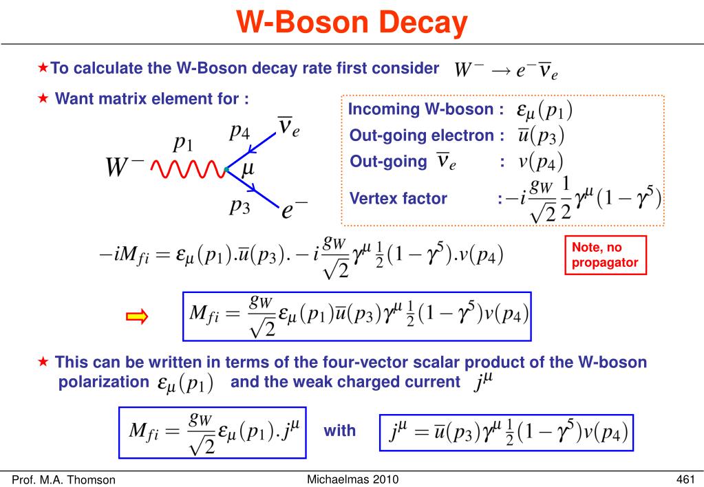
W-Boson Decay Matrix Element Calculation — This diagram shows the Feynman vertex for the decay $W^- \to e^- + \bar{\nu}_e$. The vertex factor, derived from the Lagrangian, connects the incoming W boson (with polarization $\epsilon_\mu$) to the outgoing electron (spinor $\bar{u}(p)$) and antineutrino (spinor $v(q)$). The expression for the invariant matrix element, $\mathcal{M}$, is constructed from these components.

Following the Feynman rules, the invariant matrix element $M$ for this decay is:

i M = ϵ_{μ} (k) (- i \frac{g}{2}) [u ˉ (p) γ^{μ} P_{L} v (q)]

⟹ M = - \frac{g}{2} ϵ_{μ} (k) u ˉ (p) γ^{μ} P_{L} v (q)

Here, $ϵ_{μ} (k)$ is the polarization four-vector of the incoming $W$ boson.

To find the total decay rate $Γ$ , we need to compute $∣ M ∣^{2}$ , integrate over the final state phase space, and average over the initial $W$ boson polarization states (since we typically deal with unpolarized $W$ s).

The general formula for a two-body decay rate in the rest frame of the decaying particle is:

Γ = \frac{1}{2 M _{W}} \int \frac{d ^{3} p}{( 2 π ) ^{3} 2 E _{p}} \frac{d ^{3} q}{( 2 π ) ^{3} 2 E _{q}} (2 π)^{4} δ^{(4)} (k - p - q) \frac{1}{3} pol \sum ∣ M ∣^{2}

The factor of $1/3$ comes from averaging over the three possible polarization states of the massive spin-1 $W$ boson.

2. Squaring the Matrix Element

The main task is to calculate the spin-averaged squared matrix element, $⟨ ∣ M ∣^{2} ⟩ = \frac{1}{3} \sum_{pol} ∣ M ∣^{2}$ . We sum over the final state fermion spins (which are usually not measured) and average over the initial $W$ boson polarizations.

⟨ ∣ M ∣^{2} ⟩ = \frac{1}{3} W pol \sum e, ν spins \sum - \frac{g}{2} ϵ_{μ} (k) u ˉ (p) γ^{μ} P_{L} v (q)^{2}

⟨ ∣ M ∣^{2} ⟩ = \frac{g ^{2}}{6} W pol \sum ϵ_{μ} (k) ϵ_{ν}^{*} (k) e, ν spins \sum [u ˉ (p) γ^{μ} P_{L} v (q)] [v ˉ (q) γ^{ν} P_{L} u (p)]

This expression neatly separates into a boson part and a fermion part.

2.1 The Boson Polarization Sum

For a massive spin-1 particle, the sum over its three polarization states ( $λ = 1, 2, 3$ ) is a standard result:

λ = 1 \sum 3 ϵ_{μ}^{(λ)} (k) ϵ_{ν}^{(λ) *} (k) = - g_{μν} + \frac{k _{μ} k _{ν}}{M _{W}^{2}}

This identity is crucial for calculations involving external massive vector bosons.

2.2 The Fermion Trace

The sum over the fermion spins can be converted into a trace over gamma matrices:

e, ν spins \sum \dots = Tr [s \sum u_{s} (p) u ˉ_{s} (p) γ^{μ} P_{L} r \sum v_{r} (q) v ˉ_{r} (q) (γ^{ν} P_{L})]

where $Γ = γ^{0} Γ^{†} γ^{0}$ . One can show that $γ^{ν} P_{L} = γ^{ν} P_{L}$ . Using the spin-sum identities $\sum_{s} u_{s} (p) u ˉ_{s} (p) = \neq p + m_{e}$ and $\sum_{r} v_{r} (q) v ˉ_{r} (q) = \neq q - m_{ν}$ , the trace becomes:

Fermion Part = Tr [(\neq p + m_{e}) γ^{μ} P_{L} (\neq q - m_{ν}) γ^{ν} P_{L}]

Since the electron mass ( $m_{e} \approx 0.511$ MeV) and neutrino mass ( $m_{ν} \approx 0$ ) are negligible compared to the $W$ boson mass ( $M_{W} \approx 80.4$ GeV), we can safely set them to zero. This simplifies the trace significantly:

Tr [\neq p γ^{μ} P_{L} \neq q γ^{ν} P_{L}]

Using the property $P_{L}^{2} = P_{L}$ and the cyclic property of the trace, this is equivalent to $Tr [P_{L} \neq p γ^{μ} \neq q γ^{ν}]$ . Since $P_{L} = \frac{1}{2} (1 - γ^{5})$ , and the trace of any product of an odd number of gamma matrices is zero, we get:

\frac{1}{2} Tr [\neq p γ^{μ} \neq q γ^{ν}] - \frac{1}{2} Tr [γ^{5} \neq p γ^{μ} \neq q γ^{ν}]

Using standard trace theorems:

$Tr (γ^{α} γ^{β} γ^{ρ} γ^{σ}) = 4 (g^{α β} g^{ρ σ} - g^{α ρ} g^{β σ} + g^{α σ} g^{β ρ})$
$Tr (γ^{5} γ^{α} γ^{β} γ^{ρ} γ^{σ}) = - 4 i ϵ^{α β ρ σ}$

The fermion trace evaluates to:

2 (p^{μ} q^{ν} - g^{μν} (p \cdot q) + p^{ν} q^{μ} - i ϵ^{α μ β ν} p_{α} q_{β})

2.3 Combining the Parts

Now, we contract the boson and fermion parts:

⟨ ∣ M ∣^{2} ⟩ = \frac{g ^{2}}{6} (- g_{μν} + \frac{k _{μ} k _{ν}}{M _{W}^{2}}) (Fermion Part^{μν})

In the $W$ rest frame, $k = (M_{W}, 0)$ . Kinematics gives $p \cdot q = M_{W}^{2} /2$ . After contracting all the indices (a bit of algebra!), the final result simplifies beautifully:

⟨ ∣ M ∣^{2} ⟩ = \frac{g ^{2} M _{W}^{2}}{6}

Notice how all the complicated tensor structure and dependence on individual momenta have vanished, leaving a simple constant.

4 STANDARD MODEL TREE-LEVEL PROCESSES

For a rigorous, step-by-step derivation of this result using the trace formalism, I recommend the following resource. It walks through the calculation from the matrix element to the final decay rate.

Please read section 4.2 'W-decay', starting from equation (4.16) to the end of equation (4.29). The resource uses a slightly different convention for the left-chiral projector (L = (1+γ⁵)/2), but the logic of setting up the matrix element, using spin-sum relations to get a trace (Eq. 4.27), and summing over W polarizations (Eq. 4.28) is identical. Focus on the structure of the calculation.

3. Phase Space Integration and the Final Result

With the squared matrix element in hand, we return to the decay rate formula. The two-body phase space integral simplifies to:

\int \frac{d ^{3} p}{( 2 π ) ^{3} 2 E _{p}} \frac{d ^{3} q}{( 2 π ) ^{3} 2 E _{q}} (2 π)^{4} δ^{(4)} (k - p - q) = \frac{∣ p ∣}{4 π M _{W}}

In the $W$ rest frame, for massless final particles, energy conservation gives $E_{p} + E_{q} = M_{W}$ . Momentum conservation gives $p = - q$ . Thus, $∣ p ∣ = ∣ q ∣ = M_{W} /2$ .
So, the phase space factor is $\frac{M _{W} /2}{4 π M _{W}} = \frac{1}{8 π}$ .

Putting it all together:

Γ (W^{-} \to e^{-} ν ˉ_{e}) = \frac{1}{2 M _{W}} (\frac{1}{8 π}) ⟨ ∣ M ∣^{2} ⟩ = \frac{1}{16 π M _{W}} (\frac{g ^{2} M _{W}^{2}}{6})

Γ (W^{-} \to e^{-} ν ˉ_{e}) = \frac{g ^{2} M _{W}}{96 π}

This is a clean and simple result. It's often more convenient to express this in terms of the Fermi constant, $G_{F}$ . Recall the relation derived from muon decay:
$\frac{G _{F}}{2} = \frac{g ^{2}}{8 M _{W}^{2}} ⟹ g^{2} = \frac{8 M _{W}^{2} G _{F}}{2}$
Substituting this into our expression for $Γ$ :

Γ (W^{-} \to e^{-} ν ˉ_{e}) = (\frac{8 M _{W}^{2} G _{F}}{2}) \frac{M _{W}}{96 π} = \frac{8 G _{F} M _{W}^{3}}{96 π 2}

Γ (W^{-} \to e^{-} ν ˉ_{e}) = \frac{G _{F} M _{W}^{3}}{6 π 2}

This is the final expression for the leptonic decay width of the W boson.

Test your understanding!

How would the decay rate $Γ (W^{-} \to μ^{-} ν ˉ_{μ})$ compare to $Γ (W^{-} \to e^{-} ν ˉ_{e})$ ? What principle does this illustrate?

Show answer

Since the muon mass ( $m_{μ} \approx 106$ MeV) is also negligible compared to the W boson mass, the calculation proceeds identically. Therefore, $Γ (W^{-} \to μ^{-} ν ˉ_{μ}) \approx Γ (W^{-} \to e^{-} ν ˉ_{e})$ . This is a manifestation of lepton universality in the Standard Model, which states that the electroweak force couples identically to all three generations of leptons (electron, muon, tau). The small differences observed experimentally arise from the non-zero final state masses, which we neglected.

Electroweak Unification and the W and Z Bosons

The following resource provides a slightly different but very intuitive way to arrive at the same result. Instead of using trace formalism, it calculates the matrix element for each W polarization state separately and then averages. This gives a better physical intuition for the angular distributions.

Please read through the handout from page 453 ('W-Boson Decay') to page 459. This covers the entire calculation. Pay attention to how the lepton current is evaluated in the ultra-relativistic limit and how the matrix elements for different W polarizations are calculated (pages 455-456). Notice how summing and averaging them (page 458) gives a total rate that is isotropic and matches our result.

4. Numerical Value and Total Width

Let's plug in the measured values to get a number.

$G_{F} \approx 1.166 \times 1 0^{- 5} GeV^{- 2}$
$M_{W} \approx 80.4 GeV$

Γ (W^{-} \to e^{-} ν ˉ_{e}) = \frac{( 1.166 \times 1 0 ^{- 5} GeV ^{- 2} ) ( 80.4 GeV ) ^{3}}{6 π 2} \approx 0.227 GeV

The experimentally measured value is $226.4 \pm 2.2$ MeV, so our tree-level calculation is remarkably accurate!

The W boson can also decay into $μ^{-} ν ˉ_{μ}$ and $τ^{-} ν ˉ_{τ}$ (with nearly identical rates), and into quarks. It can decay into $d u ˉ$ and $s c ˉ$ pairs. Each quark channel has 3 possible color combinations, so the rate is 3 times the leptonic rate (neglecting masses and CKM mixing effects).

3 leptonic channels: $e ν_{e}, μ ν_{μ}, τ ν_{τ}$
2 quark channels $\times$ 3 colors = 6 effective hadronic channels: $d u ˉ, s c ˉ$

So, there are a total of $3 + 6 = 9$ decay channels with roughly equal probability. The total decay width $Γ_{total}$ is approximately $9 \times Γ (W \to ℓ ν_{ℓ})$ .

Γ_{total} \approx 9 \times 0.227 GeV \approx 2.04 GeV

The measured total width is $2.085 \pm 0.042$ GeV. Again, our simple tree-level estimate is impressively close. The branching ratio (BR) to any single lepton channel is thus $BR (W \to ℓ ν_{ℓ}) = Γ_{ℓ ν} / Γ_{total} \approx 1/9 \approx 11%$ . This also agrees very well with experimental data.

Conclusion

Key Takeaways:

The decay rate of the W boson can be calculated directly from the charged-current Lagrangian using Feynman rules.
The calculation involves finding the invariant matrix element $M$ , squaring it, averaging over initial polarizations, summing over final spins, and integrating over the final state phase space.
Using trace technology and the polarization sum for a massive vector boson, the spin-averaged squared matrix element simplifies to $⟨ ∣ M ∣^{2} ⟩ = g^{2} M_{W}^{2} /6$ .
The final decay rate, $Γ (W \to ℓ ν) = G_{F} M_{W}^{3} / (6 π 2)$ , is a cornerstone prediction of the Standard Model and agrees exceptionally well with experimental measurements.
This calculation is a prime example of lepton universality and provides a way to estimate the total decay width of the W boson.

You have now completed your first full tree-level calculation in electroweak theory, from the Lagrangian to a physical observable. This is a significant milestone that connects the formal structure of QFT to the real world of particle physics experiments.

Preview of the Next Lesson:

Having tackled a decay process with the charged current, our next step will be to analyze a scattering process mediated by the neutral current. We will calculate the tree-level cross-section for neutrino-electron scattering mediated by the Z boson. This will require using the neutral-current Lagrangian we derived in the previous lesson and applying a similar set of calculational techniques.

Recommended resources