Calculating the Squared Matrix Element for Compton Scattering

Hello! Welcome back to your study of Quantum Electrodynamics.

In our last few lessons, we've successfully calculated amplitudes and cross-sections for processes like $e^{-} μ^{-} \to e^{-} μ^{-}$ and $e^{+} e^{-} \to μ^{+} μ^{-}$ . A common feature of those tree-level calculations was that they were each described by a single Feynman diagram. Today, we'll take a step up in complexity by studying a process that requires the combination of multiple diagrams: Compton scattering.

Our goal for this lesson is to calculate the unpolarized, squared matrix element for Compton scattering ( $e^{-} γ \to e^{-} γ$ ). This calculation is a classic rite of passage in QED. It will require us to handle the interference between two distinct diagrams and will give you more practice with the powerful gamma matrix trace technology you've used before.

1. The Feynman Diagrams for Compton Scattering

Compton scattering, the scattering of a photon off an electron, is described at the lowest order in perturbation theory (tree level) by two distinct processes that are quantum mechanically indistinguishable.

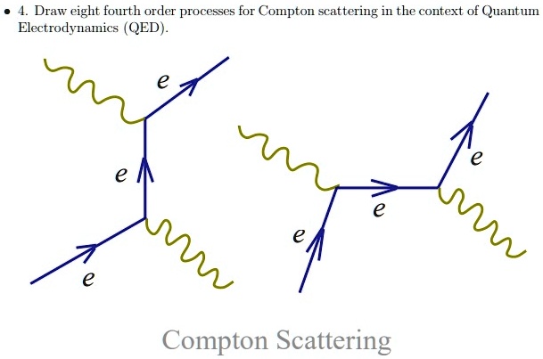
Leading-Order Feynman Diagrams for Compton Scattering — A depiction of the two leading-order Feynman diagrams for Compton scattering. On the left is the "s-channel" process, and on the right is the "t-channel" process.

Let's label the four-momenta:

Incoming electron: $p$
Incoming photon: $k$
Outgoing electron: $p^{'}$
Outgoing photon: $k^{'}$

The two diagrams represent different time-orderings of the interaction vertices:

s-channel: The incoming electron absorbs the incoming photon, propagates as a virtual (off-shell) electron with momentum $p + k$ , and then emits the outgoing photon.
t-channel: The incoming electron first emits the outgoing photon, propagates as a virtual electron with momentum $p - k^{'}$ , and then absorbs the incoming photon.

Since these two pathways lead to the same final state from the same initial state, we must sum their amplitudes before squaring to find the probability. The total matrix element is $M = M_{s} + M_{t}$ .

Using the QED Feynman rules, we can write down the amplitude for each diagram. If you'd like a quick refresher on how the S-matrix terms correspond to these diagrams, you can review the 'Compton scattering' part of the video "How To Derive The Feynman Rules For QED" by Dietterich Labs (from 33:10 to 35:30).

The individual matrix elements are:

M_{s} = u ˉ (p^{'}) (- i e γ^{ν}) ϵ_{ν}^{' *} (k^{'}) \frac{i ( \neq p + \neq k + m )}{( p + k ) ^{2} - m ^{2}} (- i e γ^{μ}) ϵ_{μ} (k) u (p)

M_{t} = u ˉ (p^{'}) (- i e γ^{μ}) ϵ_{μ} (k) \frac{i ( \neq p - \neq k ^{'} + m )}{( p - k ^{'} ) ^{2} - m ^{2}} (- i e γ^{ν}) ϵ_{ν}^{' *} (k^{'}) u (p)

Here, $ϵ_{μ} (k)$ and $ϵ_{ν}^{'} (k^{'})$ are the polarization vectors of the incoming and outgoing photons, respectively.

2. Squaring the Amplitude and Setting up the Trace

Our objective is to compute the unpolarized squared amplitude. This involves two steps:

Averaging over the two initial electron spins and two initial photon polarizations. This contributes a factor of $\frac{1}{2} \times \frac{1}{2} = \frac{1}{4}$ .
Summing over the two final electron spins and two final photon polarizations.

So, we need to compute:

⟨ ∣ M ∣^{2} ⟩ = \frac{1}{4} spins, pols \sum ∣ M_{s} + M_{t} ∣^{2} = \frac{1}{4} spins, pols \sum (∣ M_{s} ∣^{2} + ∣ M_{t} ∣^{2} + 2 Re (M_{s} M_{t}^{*}))

As you've seen before, summing over electron spins is handled by Casimir's trick, replacing the spinor products with a trace:

spins \sum ∣ M ∣^{2} \to Tr [(\neq p^{'} + m) \dots (\neq p + m) \dots]

Summing over photon polarizations uses the completeness relation. A crucial simplification arises from the gauge invariance of QED. For any amplitude involving an external photon with momentum $k$ and polarization $ϵ$ , $M = ϵ_{μ} M^{μ}$ , gauge invariance implies $k_{μ} M^{μ} = 0$ . This property, often called the Ward identity, allows us to make the simple replacement:

pols \sum ϵ_{μ} ϵ_{ν}^{*} \to - g_{μν}

This is valid when summing over the polarizations of an external photon in an S-matrix calculation.

Applying these rules, the entire expression becomes a very large trace over products of gamma matrices.

3. Evaluating the Traces

The calculation is algebraically intensive but systematic. It's a perfect example of a computation that, while lengthy by hand, follows a clear algorithm. We will follow the very explicit derivation in the "Compton Scattering" video from Dietterich Labs. The calculation is broken down into evaluating four separate traces that arise from expanding $∣ M_{s} + M_{t} ∣^{2}$ .

Compton Scattering | Klein-Nishina Formula Derivation | QED | Quantum Field Theory

The bulk of this calculation involves evaluating a series of gamma matrix traces. The video 'Compton Scattering | Klein-Nishina Formula Derivation' provides an extremely detailed, step-by-step walkthrough. We will follow its structure.

Please watch the segment from 08:41 to 22:50. This covers two main parts: Amplitude Simplification (08:41 - 11:41): Pay attention to how the denominators are simplified using p^2=m^2, k^2=0 and how the numerators are simplified using the Dirac equation (( ot{p}u(p)=mu(p))) and anticommutation relations to move gamma matrices around. This is a good warm-up. The Trace Calculation (11:41 - 22:50): This is the core of the calculation. The narrator breaks the squared amplitude into four traces: T1, T2, T3, and T4. Your goal is not to memorize every step, but to follow the logic: How are the traces set up using the completeness relations? What key gamma matrix identities are repeatedly used? (e.g., Tr(odd # of γ-matrices) = 0, ( ot{a} ot{b} = 2a\cdot b - ot{b} ot{a}), Tr(( ot{a} ot{b} ot{c} ot{d})), etc.) How is four-momentum conservation (p+k=p'+k') used to simplify dot products? Notice the symmetry argument used to get T4 from T1 and T3 from T2. This is a powerful computational shortcut.

This is a significant calculation. The key is to see the systematic application of a small number of rules:

Cyclic property of the trace: $Tr (A B C) = Tr (B C A) = Tr (C A B)$
Trace of an odd number of gamma matrices is zero.
$Tr (\neq a \neq b) = 4 (a \cdot b)$
$Tr (\neq a \neq b \neq c \neq d) = 4 [(a \cdot b) (c \cdot d) - (a \cdot c) (b \cdot d) + (a \cdot d) (b \cdot c)]$
$γ_{μ} \neq a γ^{μ} = - 2 \neq a$
$γ_{μ} \neq a \neq b γ^{μ} = 4 (a \cdot b)$
$γ_{μ} \neq a \neq b \neq c γ^{μ} = - 2 \neq c \neq b \neq a$

The calculation in the video is performed by breaking the squared amplitude into four terms, which after summation and averaging become four traces. Another excellent resource, the PDF "Compton Scattering from Quantum Electrodynamics," performs the same calculation using a slightly different organization and Mandelstam variables, which you may find illuminating to compare.

4. Assembling the Final Result

After the hard work of calculating the traces, the final step is to combine them to get the full unpolarized, squared matrix element.

Compton Scattering | Klein-Nishina Formula Derivation | QED | Quantum Field Theory

Now that the individual trace components have been calculated, let's see how they are combined to give the final expression for the unpolarized, squared matrix element.

Watch the short segment from 22:50 to 24:33. Focus on how the narrator combines the results for T1, T2, T3, and T4 and simplifies the expression. The simplified result before he introduces the 'more standard notation' in terms of frequencies is the answer to our learning objective.

Combining the simplified trace terms $X_{s} = \frac{e ^{4}}{( 2 p \cdot k ) ^{2}} T_{1}$ , $X_{t} = \frac{e ^{4}}{( 2 p \cdot k ^{'} ) ^{2}} T_{4}$ , and the interference term $X_{s t} = \frac{e ^{4}}{2 ( p \cdot k ) ( - p \cdot k ^{'} )} (T_{2} + T_{3})$ , and performing the algebra, we arrive at the final result.

The result after summing the pieces and simplifying is:

⟨ ∣ M ∣^{2} ⟩ = 2 e^{4} [\frac{p \cdot k ^{'}}{p \cdot k} + \frac{p \cdot k}{p \cdot k ^{'}} + 2 m^{2} (\frac{1}{p \cdot k} - \frac{1}{p \cdot k ^{'}}) + m^{4} (\frac{1}{p \cdot k} - \frac{1}{p \cdot k ^{'}})^{2}]

This expression is written entirely in terms of Lorentz-invariant dot products of four-momenta. This is the unpolarized, squared matrix element for Compton scattering.

Test your understanding!

Let's check the units. In natural units ( $ℏ = c = 1$ ), the matrix element $M$ is dimensionless. Therefore, $⟨ ∣ M ∣^{2} ⟩$ must also be dimensionless. We know that $e$ is dimensionless (related to $α$ ), and four-momenta have units of energy (or mass). Do the units in the final expression work out?

Show answer

Yes, they do. The term $e^{4}$ is dimensionless. Each dot product like $p \cdot k$ has units of $mass^{2}$ .

The first two terms, $\frac{p \cdot k ^{'}}{p \cdot k}$ , are ratios of $mass^{2} / mass^{2}$ , so they are dimensionless.
The third term is $m^{2} (\frac{1}{p \cdot k})$ , which has units of $mass^{2} \times \frac{1}{mass ^{2}}$ , making it dimensionless.
The last term is $m^{4} (\frac{1}{p \cdot k})^{2}$ , which has units of $mass^{4} \times \frac{1}{( mass ^{2} ) ^{2}}$ , also dimensionless.
All terms are consistent and the final expression is dimensionless, as expected.

Conclusion

In this lesson, you have tackled one of the most important canonical calculations in QED. The algebraic complexity is significant, but the underlying process is a straightforward application of the tools you've been developing.

Key Takeaways:

Compton scattering at tree level is described by the sum of an s-channel and a t-channel Feynman diagram, and their amplitudes interfere.
Calculating the unpolarized, squared amplitude involves averaging over initial states, summing over final states, and evaluating traces of gamma matrices.
Gauge invariance ( $k_{μ} M^{μ} = 0$ ) is a crucial physical principle that simplifies the sum over photon polarizations to $\sum ϵ_{μ} ϵ_{ν}^{*} = - g_{μν}$ .
The final amplitude, expressed in Lorentz-invariant dot products, contains all the dynamical information of the scattering process at tree level.

Preview of the Next Lesson:
We are now in the same position as we were at the start of the previous lesson: we have the squared matrix element $⟨ ∣ M ∣^{2} ⟩$ , but not a directly measurable cross-section. In the next lesson, we will take the expression we just derived, evaluate it in the laboratory frame (where the electron is initially at rest), perform the phase space integration, and derive the famous Klein-Nishina formula for the differential cross-section of Compton scattering.

Recommended resources

1. The Feynman Diagrams for Compton Scattering

2. Squaring the Amplitude and Setting up the Trace

3. Evaluating the Traces

4. Assembling the Final Result

Conclusion