Klein-Nishina Formula Derivation

Hello! Welcome back to your exploration of Quantum Electrodynamics.

In our previous lesson, you accomplished the demanding task of calculating the unpolarized, squared matrix element, $⟨ ∣ M ∣^{2} ⟩$ , for Compton scattering. This gave us a Lorentz-invariant expression containing the core dynamics of the interaction.

Today, we will connect that abstract result to the real world. Our goal is to derive the Klein-Nishina formula for the differential cross-section of Compton scattering ( $e^{-} γ \to e^{-} γ$ ). This involves taking our expression for $⟨ ∣ M ∣^{2} ⟩$ , combining it with the general formula for a cross-section, and evaluating the result in the laboratory frame to arrive at one of the hallmark predictions of QED.

1. From Matrix Element to Cross-Section

Let's begin by briefly recalling our starting points. From the last lesson, the spin- and polarization-averaged squared matrix element for Compton scattering is:

⟨ ∣ M ∣^{2} ⟩ = 2 e^{4} [\frac{p \cdot k ^{'}}{p \cdot k} + \frac{p \cdot k}{p \cdot k ^{'}} + 2 m^{2} (\frac{1}{p \cdot k} - \frac{1}{p \cdot k ^{'}}) + m^{4} (\frac{1}{p \cdot k} - \frac{1}{p \cdot k ^{'}})^{2}]

where $p, k$ are the initial electron and photon four-momenta, and $p^{'}, k^{'}$ are the final ones.

The general formula for the differential cross-section of a 2-particle to 2-particle scattering process ( $1 + 2 \to 3 + 4$ ) is:

d σ = \frac{1}{4 ( p _{1} \cdot p _{2} ) ^{2} - m _{1}^{2} m _{2}^{2}} ⟨ ∣ M ∣^{2} ⟩ (2 π)^{4} δ^{4} (p_{1} + p_{2} - p_{3} - p_{4}) \frac{d ^{3} p _{3}}{( 2 π ) ^{3} 2 E _{3}} \frac{d ^{3} p _{4}}{( 2 π ) ^{3} 2 E _{4}}

The term in the denominator is related to the incident flux. The rest of the expression is the Lorentz-invariant phase space element for the final state particles, weighted by the squared matrix element and constrained by four-momentum conservation.

A thorough derivation of this formula from first principles is quite involved. For our purposes, the following resource provides a clear outline of the key steps.

3.3 cross-sections

The PDF '3.3 cross-sections' outlines the derivation of the general Lorentz-invariant formula for the cross-section. It connects the S-matrix element to the transition rate and then to the cross-section by considering incident flux and density of states.

Please read the first three pages of this document, from the beginning of section §3.3 down to equation (3.3.30). Focus on understanding how the pieces come together: the transition rate per unit volume (Eq. 3.3.14), the density of final states (Eq. 3.3.17), and the flux factor (Eq. 3.3.29), leading to the final Lorentz-invariant expression for d\sigma.

2. Kinematics in the Laboratory Frame

To get the Klein-Nishina formula, we must evaluate the general cross-section formula in a specific reference frame: the laboratory frame, where the initial electron is at rest.

Initial electron: $p = (m, 0)$
Initial photon: $k = (ω, k)$ with $∣ k ∣ = ω$
Final electron: $p^{'} = (E^{'}, p^{'})$
Final photon: $k^{'} = (ω^{'}, k^{'})$ with $∣ k^{'} ∣ = ω^{'}$

The angle $θ$ between the incoming and outgoing photons is defined by $k \cdot k^{'} = ∣ k ∣∣ k^{'} ∣ cos θ = ω ω^{'} cos θ$ .

First, let's simplify the flux factor in our cross-section formula, $4 (p \cdot k)^{2} - m_{e}^{2} m_{γ}^{2}$ . Since the photon is massless ( $m_{γ} = 0$ ) and $p \cdot k = mω$ , the flux factor becomes simply $4 mω$ .

The differential cross-section formula for Compton scattering in the lab frame is thus:

d σ = \frac{1}{4 mω} ⟨ ∣ M ∣^{2} ⟩ \frac{1}{( 2 π ) ^{2}} \int \frac{d ^{3} p ^{'}}{2 E ^{'}} \frac{d ^{3} k ^{'}}{2 ω ^{'}} δ^{4} (p + k - p^{'} - k^{'})

Our task is to perform the phase space integral to find $\frac{d σ}{d Ω}$ , where $d Ω$ is the solid angle of the outgoing photon.

3. Integrating the Phase Space

The next step is algebraically intensive but follows a standard procedure. We use the delta functions to eliminate integration variables until only the desired differential, $d Ω$ , remains.

The full derivation is quite detailed. The following resources walk through this calculation explicitly.

3.3 cross-sections

The document '3.3 cross-sections' continues by applying the general formula specifically to Compton scattering in the lab frame. It carefully performs the phase space integration.

Read from the subsection on Compton scattering (just below Eq. 3.3.32) down to Eq. (3.3.52). Pay close attention to how the phase space integral is reduced. The key steps are: Integrating over d^3p' using the 3-momentum delta function. Writing d^3k' in spherical coordinates to isolate d\Omega. Using the properties of the Dirac delta function to perform the integral over d|\vec{k}'| = d\omega', which requires calculating a derivative of the delta function's argument (Eq. 3.3.45). Deriving the famous Compton scattering formula (Eq. 3.3.49) relating \omega' to \omega and heta.

For a slightly different perspective that arrives at the same point, you can also consult the resource "Compton Scattering from Quantum Electrodynamics".

Compton Scattering from Quantum Electrodynamics

This document, 'Compton Scattering from Quantum Electrodynamics', provides an alternative derivation of the lab frame cross-section, starting from the Lorentz-invariant phase space integral.

This is an optional reading. Skim through Section 3.2 'Lab Frame' (pages 6-7). Notice how it reaches the same result (Eq. 3.24) as the previous resource, showing the robustness of the method. The key takeaway is the final relationship between d\sigma and (\langle|\mathcal{M}|^2 angle) after phase space integration.

After performing the integration, we arrive at the following crucial link between the differential cross-section and the matrix element:

\frac{d σ}{d Ω} = \frac{1}{( 8 π ) ^{2}} (\frac{ω ^{'}}{ω m})^{2} ⟨ ∣ M ∣^{2} ⟩

where the outgoing photon energy $ω^{'}$ is now fixed by the scattering angle $θ$ via the Compton formula:

ω^{'} = \frac{ω}{1 + \frac{ω}{m} ( 1 - cos θ )}

4. Assembling the Klein-Nishina Formula

We have all the ingredients. The final step is to take our expression for $⟨ ∣ M ∣^{2} ⟩$ , evaluate its dot products in the lab frame, and substitute it into the formula for $\frac{d σ}{d Ω}$ .

First, let's evaluate the dot products in the lab frame:

$p \cdot k = mω$
$p \cdot k^{'} = m ω^{'}$
From four-momentum conservation, $p + k = p^{'} + k^{'}$ , we can write $p \cdot k^{'} = p^{'} \cdot k$ . This is useful for some forms of the amplitude.

Substitute these into the expression for $⟨ ∣ M ∣^{2} ⟩$ :

⟨ ∣ M ∣^{2} ⟩ = 2 e^{4} [\frac{m ω ^{'}}{mω} + \frac{mω}{m ω ^{'}} + 2 m^{2} (\frac{1}{mω} - \frac{1}{m ω ^{'}}) + m^{4} (\frac{1}{mω} - \frac{1}{m ω ^{'}})^{2}]

Simplifying gives:

⟨ ∣ M ∣^{2} ⟩ = 2 e^{4} [\frac{ω ^{'}}{ω} + \frac{ω}{ω ^{'}} + 2 m (\frac{1}{ω} - \frac{1}{ω ^{'}}) + m^{2} (\frac{1}{ω} - \frac{1}{ω ^{'}})^{2}]

Now, we can use the Compton formula, which can be rearranged as $\frac{1}{ω ^{'}} - \frac{1}{ω} = \frac{1 - c o s θ}{m}$ , to simplify the terms in the parentheses:

⟨ ∣ M ∣^{2} ⟩ = 2 e^{4} [\frac{ω ^{'}}{ω} + \frac{ω}{ω ^{'}} - 2 m (\frac{1 - cos θ}{m}) + m^{2} (\frac{1 - cos θ}{m})^{2}]

= 2 e^{4} [\frac{ω ^{'}}{ω} + \frac{ω}{ω ^{'}} - 2 (1 - cos θ) + (1 - cos θ)^{2}]

= 2 e^{4} [\frac{ω ^{'}}{ω} + \frac{ω}{ω ^{'}} - (2 - 2 cos θ) + (1 - 2 cos θ + cos^{2} θ)]

= 2 e^{4} [\frac{ω ^{'}}{ω} + \frac{ω}{ω ^{'}} - 1 + cos^{2} θ] = 2 e^{4} [\frac{ω ^{'}}{ω} + \frac{ω}{ω ^{'}} - sin^{2} θ]

This is a remarkably compact form for the squared amplitude in the lab frame.

Now, substitute this back into our expression for $\frac{d σ}{d Ω}$ :

\frac{d σ}{d Ω} = \frac{1}{64 π ^{2}} (\frac{ω ^{'}}{ω m})^{2} (2 e^{4} [\frac{ω ^{'}}{ω} + \frac{ω}{ω ^{'}} - sin^{2} θ])

Using the fine-structure constant $α = \frac{e ^{2}}{4 π}$ , which means $e^{4} = 16 π^{2} α^{2}$ , we get:

\frac{d σ}{d Ω} = \frac{2 \cdot 16 π ^{2} α ^{2}}{64 π ^{2} m ^{2}} (\frac{ω ^{'}}{ω})^{2} [\frac{ω ^{'}}{ω} + \frac{ω}{ω ^{'}} - sin^{2} θ]

\frac{d σ}{d Ω} = \frac{α ^{2}}{2 m ^{2}} (\frac{ω ^{'}}{ω})^{2} (\frac{ω}{ω ^{'}} + \frac{ω ^{'}}{ω} - sin^{2} θ)

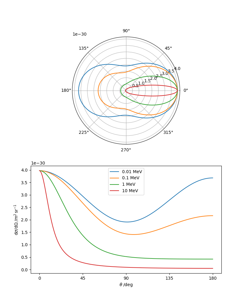
This is the Klein-Nishina formula, a historic achievement of early QED.

Test your understanding!

Consider the low-energy (non-relativistic) limit, where the incoming photon energy is much less than the electron's rest mass, $ω ≪ m$ . What does the Klein-Nishina formula reduce to in this limit?

Hint: In this limit, the electron recoil is negligible, so $ω^{'} \approx ω$ .

Show answer

If $ω^{'} \approx ω$ , the Klein-Nishina formula becomes:

\frac{d σ}{d Ω} \approx \frac{α ^{2}}{2 m ^{2}} (\frac{ω}{ω})^{2} (\frac{ω}{ω} + \frac{ω}{ω} - sin^{2} θ)

= \frac{α ^{2}}{2 m ^{2}} (1 + 1 - sin^{2} θ) = \frac{α ^{2}}{2 m ^{2}} (2 - sin^{2} θ) = \frac{α ^{2}}{2 m ^{2}} (1 + cos^{2} θ)

This is the formula for Thomson scattering, which describes the classical scattering of electromagnetic radiation by a free charged particle. It's reassuring that the quantum field theory result correctly reproduces the classical result in the appropriate limit.

The energy dependence of the scattering is illustrated beautifully in the following plot.

Klein-Nishina Differential Cross-Section for Compton Scattering — Polar (top) and Cartesian (bottom) plots of the Klein-Nishina differential cross-section for various incident photon energies. At low energy (0.01 MeV, blue), the distribution is nearly symmetric, approaching the classical Thomson limit. At high energy (10 MeV, red), the scattering is strongly peaked in the forward direction.

Conclusion

Congratulations on deriving the Klein-Nishina formula! This is a cornerstone result that demonstrates the predictive power of QED. It was one of the first calculations in QED that could be compared directly with high-precision experiments, and its success was a major validation of the theory.

Key Takeaways:

The differential cross-section $d σ / d Ω$ is derived by combining the squared matrix element $⟨ ∣ M ∣^{2} ⟩$ with the Lorentz-invariant phase space element and evaluating the result in a specific reference frame.
The kinematics of Compton scattering in the lab frame lead to the famous Compton formula, which relates the scattered photon's energy to its scattering angle.
The final Klein-Nishina formula accurately describes the angular distribution of scattered photons and its dependence on the incident photon energy.
In the low-energy limit, the Klein-Nishina formula correctly reduces to the classical Thomson scattering cross-section.

Preview of the Next Lesson:
So far, we have been expressing our results in terms of dot products like $p \cdot k$ . While Lorentz-invariant, this can sometimes obscure the physics in high-energy collisions. In the next lesson, we will introduce the Mandelstam variables (s, t, u), which provide a powerful and conventional way to express scattering amplitudes for 2-to-2 processes in a manifestly Lorentz-invariant and symmetric form.

Recommended resources

1. From Matrix Element to Cross-Section

2. Kinematics in the Laboratory Frame

3. Integrating the Phase Space

4. Assembling the Klein-Nishina Formula

Conclusion