Calculating the Squared Matrix Element for e⁻μ⁻ Scattering

1. The Amplitude for Electron-Muon Scattering

Let's consider the scattering process $e^{-}(p_a)+{\mu }^{-}(p_b)\to e^{-}(p_c)+{\mu }^{-}(p_d)$, where $p_i$ are the respective 4-momenta. At the lowest order in the electromagnetic coupling, this process is mediated by the exchange of a single virtual photon.

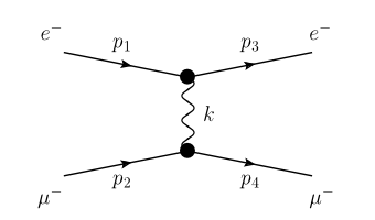
From the Feynman rules you learned previously, we can write down the invariant amplitude $\mathcal{M}$ for this diagram. It consists of the electron current, the muon current, and the photon propagator connecting them.

The amplitude, $i\mathcal{M}$, is:

where $q=p_a-p_c$ is the momentum of the exchanged photon. Cleaning this up, we get:

This expression depends on the specific initial and final spin states of the electron and muon, which are contained within the spinors $u$ and $\bar{u}$.

2. Unpolarized Scattering and Spin Sums

In most real-world experiments, the incoming beams are unpolarized, meaning they contain an equal mix of spin-up and spin-down particles. Furthermore, detectors are usually insensitive to the spins of the outgoing particles. Therefore, to get a physically relevant quantity, we must:

1. Average over the possible initial spin states.
2. Sum over all possible final spin states.

For this process, we have 2 initial electron spins and 2 initial muon spins, giving 4 possible initial spin combinations. We average by dividing by 4. The quantity we need to compute is:

To evaluate this, we first need $|\mathcal{M}{|}^2=\mathcal{M}{\mathcal{M}}^{\ast }$. The following resource walks through the first few steps: finding the complex conjugate ${\mathcal{M}}^{\ast }$ and setting up the spin-summed expression.

As you've just read, the squared amplitude can be written as the product of two tensors, one for the electron line and one for the muon line:

Our task is now to compute the spin sum of this expression. This looks formidable, as it involves products of eight spinors.

3. Casimir's Trick: From Spinors to Traces

This is where a powerful technique known as Casimir's Trick comes in. The trick uses the spin sum completeness relations for Dirac spinors to convert the sum over spin states into a trace over gamma matrices. The key relations are:

These relations are themselves 4x4 matrices.

Let's see how this works for the electron tensor $L_{(e)}^{\mu \nu }$. When we sum over the electron spins $s_a$ and $s_c$, we get:
\begin{align*}
\sum_{s_a, s_c} L^{\mu\nu}{(e)} &= \sum{s_a, s_c} \left[ \bar{u}(p_c, s_c)\gamma^\mu u(p_a, s_a) \right] \left[ \bar{u}(p_a, s_a)\gamma^\nu u(p_c, s_c) \right] \
&= \sum_{s_c} \bar{u}(p_c, s_c)\gamma^\mu \left( \sum_{s_a} u(p_a, s_a) \bar{u}(p_a, s_a) \right) \gamma^\nu u(p_c, s_c) \
&= \sum_{s_c} \bar{u}(p_c, s_c)\gamma^\mu (\not p_a + m_e) \gamma^\nu u(p_c, s_c)
\end{align*}
Writing out the spinor indices makes the final step clear:
\begin{align*}
& \quad \sum_{s_c} \bar{u}{\alpha}(p_c, s_c) \left[\gamma^\mu (\not p_a + m_e) \gamma^\nu\right]{\alpha\beta} u_{\beta}(p_c, s_c) \
&= \sum_{s_c} \left[\gamma^\mu (\not p_a + m_e) \gamma^\nu\right]{\alpha\beta} u{\beta}(p_c, s_c) \bar{u}{\alpha}(p_c, s_c) \
&= \left[\gamma^\mu (\not p_a + m_e) \gamma^\nu\right]{\alpha\beta} \left[\not p_c + m_e\right]_{\beta\alpha} \
&= \text{Tr}\left[ \gamma^\mu (\not p_a + m_e) \gamma^\nu (\not p_c + m_e) \right]
\end{align*}
In the second line, we used the fact that the term in brackets is a matrix and the spinors are just numbers (for fixed indices), so we can reorder them. In the third line, we applied the spin sum relation for the outgoing electron. The final expression is a trace, which is a sum over diagonal elements (${\sum }_{\alpha }{M}_{\alpha \alpha }$).

This is the essence of Casimir's trick. The reading from LINK on page 93 (eq. 5.6) shows this exact transformation. Similarly, the slide below provides a general statement of the trick.

So, our spin-averaged squared amplitude becomes a product of two traces:

Note: We've used the cyclic property of the trace ($\text{Tr}(ABC)=\text{Tr}(BCA)$) to rearrange the first trace into a more standard form.

4. Gamma Matrix Trace Technology

Our problem is now reduced to calculating traces of products of gamma matrices. This is a standard procedure in QFT, and there is a set of "trace theorems" that allow us to evaluate them systematically.

A concise list of the most important theorems is provided in the following resource.

While having these formulas is useful, your background in physics and mathematics suggests you'll appreciate knowing where they come from. They all derive from the fundamental Clifford algebra, $\{{\gamma }^{\mu },{\gamma }^{\nu }\}=2{\eta }^{\mu \nu }$, and the cyclic property of the trace. The following video provides detailed derivations.

The most important result for us is the trace of four gamma matrices:

5. The Final Calculation

We have all the tools. Now we just need to assemble the pieces. We must calculate the electron trace, $T_{(e)}^{\mu \nu }=\text{Tr}\left[(/p_c+m_e){\gamma }^{\mu }(/p_a+m_e){\gamma }^{\nu }\right]$, and the muon trace, and then contract them.

The entire calculation is laid out for you in the resource we've been following. Your task is to work through it carefully, using the trace theorems you've just learned.

The final result, after performing the traces and contracting the indices, is:

where $q^2=(p_a-p_c{)}^2$.

Conclusion

In this lesson, we performed our first full calculation of a physical quantity in QED. You learned the essential techniques for handling spin in unpolarized scattering processes, which are central to almost all practical QFT calculations.

Key Takeaways:

• To calculate unpolarized cross-sections, we must average over initial spins and sum over final spins.
• Casimir's Trick is a crucial technique that converts these difficult spin sums into traces of gamma matrices, using the identity ${\sum }_s{u}^s(p){\bar{u}}^s(p)=/p+m$.
• Trace theorems provide a systematic algebra for evaluating traces of products of gamma matrices, all stemming from the Clifford algebra.
• The final squared amplitude is a Lorentz-invariant scalar, expressed in terms of 4-vector dot products and masses.

Preview of the Next Lesson:
With these powerful tools in hand, we are ready to tackle other QED processes. In the next lesson, we will calculate the unpolarized, squared matrix element for electron-positron annihilation into a muon-antimuon pair: $e^{+}{e}^{-}\to {\mu }^{+}{\mu }^{-}$. This will give you more practice with trace technology and introduce a different kinematic channel (s-channel vs. t-channel) and the use of v-spinors for antiparticles.