Feynman Rules for Tree-Level QED

1. From Lagrangian to Diagrams: A Conceptual Framework

The Feynman rules don't appear out of thin air. They are a clever distillation of the results from applying perturbation theory to our QED Lagrangian. As you saw in Module 2 with ${\varphi }^4$ theory, calculating scattering amplitudes involves:

1. Expanding the S-matrix operator using the Dyson series: $S=T\left\{\exp \left(i\int d^{4}x{\mathcal{L}}_{\text{int}}\right)\right\}$.
2. Using Wick's theorem to decompose the time-ordered products of fields into normal-ordered products and propagators.
3. Evaluating the matrix elements of these terms between initial and final particle states.

In QED, this process is significantly more complex due to the vector and spinor nature of the fields. However, the result is a beautifully systematic set of rules, one for each component of a diagram: external particles, internal propagating particles, and interaction vertices.

A key convention in these diagrams is how we distinguish particles from antiparticles. The arrows on fermion lines follow the flow of electron number (charge), not necessarily the direction of motion in time.

• An electron (charge -e) carries electron number +1. Its arrow points forward in time.
• A positron (charge +e) carries electron number -1. It is represented as an electron number of +1 flowing backward in time. Thus, its arrow points backward along its direction of motion.

This clever convention ensures that electron number is conserved at every vertex; an arrow always flows continuously through a fermion line.

To see a clear explanation of this crucial convention, please watch the following segment.

2. The Complete Feynman Rules for QED

Let's now assemble the complete set of rules. Each rule is a factor that we write down when we see the corresponding feature in a diagram. To get the total amplitude for a diagram, we multiply all these factors together.

Visual Summary

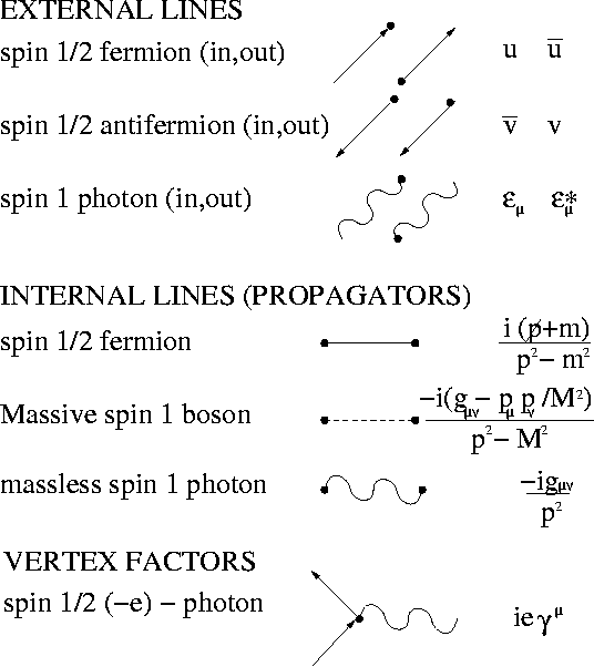
The following image provides a concise graphical summary of the core rules for QED. We will break down each component in detail below.

The Rules in Detail

We'll work in momentum space and use natural units ($\hslash =c=1$). The fine-structure constant is $\alpha =e^2/4\pi$.

1. External Lines (Asymptotic States)
These factors represent the wavefunctions of the incoming and outgoing particles.

• Incoming electron: $u^s(p)$
• Outgoing electron: ${\bar{u}}^s(p)$
• Incoming positron: ${\bar{v}}^s(p)$
• Outgoing positron: $v^s(p)$
• Incoming photon: ${ϵ}_{\mu }^{\lambda }(k)$
• Outgoing photon: ${ϵ}_{\mu }^{\lambda \ast }(k)$

Here, $p$ and $k$ are the 4-momenta, $s$ is the spin state, and $\lambda$ is the polarization.

2. Internal Lines (Propagators)
These factors describe the propagation of a "virtual" particle between two vertices.

• Fermion (electron/positron) Propagator: A solid line with momentum $p$.
  $\frac{i(/p+m)}{p^2-m^2+iϵ}$
  where $/p={\gamma }^{\mu }{p}_{\mu }$. This is the Feynman propagator for the Dirac field which we derived previously.

• Photon Propagator: A wavy line with momentum $k$. In the Feynman gauge, which we will use, this takes a simple, Lorentz-invariant form:
  $\frac{-i{\eta }_{\mu \nu }}{k^2+iϵ}$

3. Vertex
This is the point where lines meet, representing the interaction ${\mathcal{L}}_{\text{int}}=-e\bar{\psi }{\gamma }^{\mu }\psi A_{\mu }$.

• QED Vertex: A junction of one photon line and two fermion lines. The factor is:
  $-ie{\gamma }^{\mu }$
  The factor of $-i$ comes from the $i$ in the exponential of the S-matrix expansion, $S\approx 1+i\int {\mathcal{L}}_{\text{int}}$.

4. Conservation and Integration

• For each vertex, impose 4-momentum conservation. The sum of incoming momenta must equal the sum of outgoing momenta.
• For any undetermined ("loop") momentum $k$ that remains after enforcing conservation at all vertices, integrate over it: $\int \frac{d^{4}k}{(2\pi {)}^4}$. (This applies to loop diagrams, which we'll study later, not tree-level diagrams).

5. Fermionic Signs and Matrix Ordering

This is a subtle but critical set of rules arising from the anti-commuting nature of fermion fields.

• Dirac Matrix Ordering: For a continuous fermion line, write the Dirac-matrix-valued factors (spinors, propagators, vertices) from right to left as you follow the line from its "head" (where the arrow terminates) to its "tail" (where the arrow begins). This corresponds to following the fermion line against the direction of its arrow.
• Relative Signs:
  • Add a relative minus sign between two diagrams that differ only by the exchange of two identical external fermion lines (e.g., swapping the two outgoing electrons in Møller scattering, $e^{-}{e}^{-}\to e^{-}{e}^{-}$).
  • Include a factor of $-1$ for every closed fermion loop.

The following resource provides a very clear and comprehensive list of these rules, with excellent explanations of the trickier points like matrix ordering and sign conventions.

3. Justification and Derivation

Stating these rules is one thing, but knowing where they come from is another. While a full derivation of every rule is extensive, we can highlight the physical reasoning behind the most important ones. The process involves calculating the S-matrix element for a given process and then comparing the resulting mathematical expression with the diagram we draw for it. By identifying patterns across many different processes, the rules can be "read off".

This painstaking procedure is exactly what is performed in the video below. You are not required to watch it in its entirety, but it serves as an excellent reference for the complete, rigorous derivation that underpins the rules we use. The final segment is particularly enlightening, as it brings everything together.

A particularly subtle point is the form of the photon propagator. Its form depends on the gauge choice. However, for S-matrix calculations, we can use the simple Feynman gauge form because the additional, more complex terms ultimately do not contribute to physical amplitudes due to current conservation. This is a consequence of the Ward-Takahashi identity. The following reading demonstrates this for a tree-level diagram.

Conclusion

In this lesson, you have learned the complete set of Feynman rules for tree-level calculations in Quantum Electrodynamics. These rules are the bridge between the formal Lagrangian of a theory and its observable predictions.

Key Takeaways:

• Feynman rules provide a dictionary to translate diagrams into mathematical amplitudes.
• External lines are represented by spinors ($u,v,\bar{u},\bar{v}$) for fermions and polarization vectors (${ϵ}_{\mu }$) for photons.
• Internal lines are represented by propagators, which for fermions and photons in Feynman gauge are $\frac{i(/p+m)}{p^2-m^2}$ and $\frac{-i{\eta }_{\mu \nu }}{k^2}$ respectively.
• The QED vertex gives a factor of $-ie{\gamma }^{\mu }$.
• The anti-commuting nature of fermions imposes strict rules on matrix ordering (write factors right-to-left against the fermion arrow) and relative signs for exchanged identical fermions.

Preview of the Next Lesson:
We now have the complete recipe book. In our next session, we will immediately put it to use to calculate our first full QED process: the scattering of an electron and a muon ($e^{-}{\mu }^{-}\to e^{-}{\mu }^{-}$). This will require us to learn the powerful computational techniques of Casimir's trick and gamma matrix trace technology, which are essential for dealing with the spin sums in unpolarized scattering experiments.