Price Elasticity of Supply: Definition, Calculation, and Determinants

Introduction

Welcome to your next lesson on the topic of elasticity. In our previous sessions, we have thoroughly explored elasticity from the demand side, looking at how quantity demanded responds to changes in a product's own price, consumer income, and the price of related goods. We established a consistent analytical method: define the concept, learn its formula, interpret the result, and understand its practical implications.

Today, we pivot our focus from the consumer to the producer. This lesson is designed to address the learning outcome: Define and calculate price elasticity of supply and explain its determinants. We will investigate how responsive producers are to changes in market price, a concept known as the price elasticity of supply (PES).

Understanding supply-side responsiveness is just as critical as understanding the demand side. It helps analysts predict how markets will react to shocks, how quickly production can ramp up or down, and what factors constrain a firm's ability to meet market demand. For the CFA exam, this is a core microeconomic principle.

1. Defining and Calculating Price Elasticity of Supply

Price elasticity of supply (PES) measures the degree of responsiveness of the quantity supplied of a good to a change in that good's price. In simple terms, it tells us how much more (or less) of a product firms are willing and able to sell when its price goes up (or down).

The formula is analogous to what we've seen before:

$E_{S} = \frac{Percentage Change in Quantity Supplied}{Percentage Change in Price} = \frac{%Δ Q _{S}}{%Δ P}$

A key difference from demand elasticities is that PES is always a positive number. This is a direct consequence of the Law of Supply: as price increases, quantity supplied increases, so both the numerator and denominator have the same sign. Therefore, our interpretation will focus on the magnitude of the number, not its sign.

Let's watch a short video to establish the foundations of PES, including its formula, interpretation, and a worked-out calculation.

Y1 12) Price Elasticity of Supply (PES)

This video from EconplusDal provides a clear and concise introduction to Price Elasticity of Supply (PES). It covers the core definition, the formula, the different classifications of elasticity, and a straightforward calculation example.

Watch the video from the beginning until 02:51. Focus on: The definition and formula for PES. The reason why the result is always positive. The classification of supply based on the PES value (e.g., inelastic, elastic). How to perform the calculation using the oil price example.

Interpreting the PES Value

As the video explained, we classify supply elasticity based on its magnitude:

Elastic Supply ( $E_{S} > 1$ ): The percentage change in quantity supplied is greater than the percentage change in price. This indicates that producers are highly responsive to price changes.
Inelastic Supply ( $0 < E_{S} < 1$ ): The percentage change in quantity supplied is less than the percentage change in price. Producers are not very responsive to price changes.
Unit Elastic Supply ( $E_{S} = 1$ ): The percentage change in quantity supplied is equal to the percentage change in price.

There are also two theoretical extremes:

Perfectly Inelastic Supply ( $E_{S} = 0$ ): Quantity supplied does not change at all, regardless of the change in price.
Perfectly Elastic Supply ( $E_{S} = \infty$ ): Producers will supply any amount at a specific price, but will supply zero at any price below that.

Let's solidify this with a quick practice problem.

Practice Question:
The price of silver increases from $20 to $22 per ounce. In response, a mining company increases its monthly production from 100,000 ounces to 105,000 ounces. Calculate and interpret the price elasticity of supply.

Solution:

Calculate the percentage change in price:
$%Δ P = \frac{$22 - $20}{$20} \times 100% = \frac{$2}{$20} \times 100% = 10%$
Calculate the percentage change in quantity supplied:
$%Δ Q_{S} = \frac{105 , 000 - 100 , 000}{100 , 000} \times 100% = \frac{5 , 000}{100 , 000} \times 100% = 5%$
Calculate PES:
$E_{S} = \frac{5%}{10%} = 0.5$

Interpretation: Since $E_{S} = 0.5$ (which is less than 1), the supply of silver in this scenario is inelastic. The 10% increase in price led to a proportionally smaller (5%) increase in quantity supplied.

2. The Graphical Representation of PES

Just as with demand, the elasticity of supply has a clear graphical representation. The slope of the supply curve provides a visual cue:

A steep supply curve indicates inelastic supply.
A flat or shallow supply curve indicates elastic supply.

This visual distinction is powerfully illustrated in the following image.

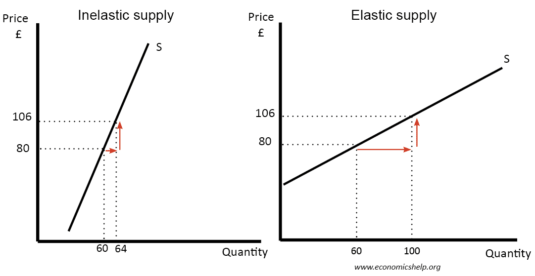
Inelastic vs. Elastic Supply Curves — This image contrasts an inelastic (steep) supply curve on the left with an elastic (shallow) supply curve on the right. Notice how the same price increase leads to a much larger change in quantity supplied for the elastic curve.

For the CFA exam, it's also useful to know a rule of thumb based on where a linear supply curve intersects the axes.

Price Elasticity of Supply on a Graph Explained

The shape and position of the supply curve on a graph provide quick clues about its elasticity. This resource explains a very helpful rule for interpreting graphs, which is a valuable skill for exams.

Please read the section titled 'Price Elasticity of Supply on a Graph Video Summary'. Pay close attention to the descriptions of how each type of supply elasticity is represented on a graph. The tips on where the curve intersects the axes are particularly important.

Let's summarize these crucial graphical rules:

Perfectly Inelastic ( $E_{S} = 0$ ): A vertical line. Quantity is fixed.
Inelastic ( $E_{S} < 1$ ): An upward-sloping line that intersects the horizontal (quantity) axis.
Unit Elastic ( $E_{S} = 1$ ): An upward-sloping line that passes through the origin (0,0).
Elastic ( $E_{S} > 1$ ): An upward-sloping line that intersects the vertical (price) axis.
Perfectly Elastic ( $E_{S} = \infty$ ): A horizontal line. Price is fixed.

3. Determinants of Price Elasticity of Supply

Now we turn to the "why" behind the numbers. What makes the supply of one good highly elastic, while another is stubbornly inelastic? Several factors determine a firm's ability to adjust its production in response to price changes.

Price Elasticity of Supply Explained I A Level and IB Economics

This video from tutor2u provides a detailed breakdown of the key factors that determine price elasticity of supply. Understanding these determinants is crucial for analyzing real-world market behavior.

Watch the section from 01:57 to 05:00. This part covers the main determinants of PES. As you watch, think about how each factor affects a firm's ability to change its production level quickly.

To structure this information for effective recall, let's summarize the key determinants of PES in a table.

Determinant	Impact on Elasticity	Explanation
Time Horizon	Supply is more elastic in the long run.	In the short run, at least one factor of production is fixed (e.g., factory size). In the long run, firms can adjust all inputs, such as building new facilities, making supply more responsive.
Spare Production Capacity	Firms with more spare capacity have more elastic supply.	If a factory is only running at 70% capacity, it can easily increase output without incurring large costs. A firm at 100% capacity has very inelastic supply in the short run.
Level of Inventories	Firms with high levels of inventory (stocks) have more elastic supply.	If a firm has a warehouse full of finished goods, it can respond to a price increase instantly by selling its stock. This applies mainly to non-perishable goods.
Factor Mobility / Substitutability	The easier it is to move resources (labor, capital) into production, the more elastic supply is.	If a farmer can easily switch from growing corn to soybeans when soybean prices rise, the supply of soybeans is more elastic. Similarly, if workers can easily be retrained, supply is more elastic.
Complexity of Production	Goods that are simpler and quicker to produce have more elastic supply.	Producing a t-shirt is fast and simple, so supply is relatively elastic. Building a commercial airplane takes years and specialized equipment, making its supply highly inelastic.

Conclusion

In this lesson, we completed our survey of the fundamental elasticity concepts by focusing on the producer's side. We defined price elasticity of supply, learned how to calculate and interpret it, visualized it on a graph, and, critically, understood the underlying factors that determine it.

Key Takeaways:

Price Elasticity of Supply (PES) measures the responsiveness of quantity supplied to a price change. Its formula is $E_{S} = %Δ Q_{S} /%Δ P$ .
PES is always positive. We interpret its magnitude: $E_{S} > 1$ is elastic, and $E_{S} < 1$ is inelastic.
Graphically, a steep supply curve is inelastic, while a flat curve is elastic. Where the curve intersects the axes provides a shortcut for identifying its elasticity.
The key determinants of PES are the time horizon, spare capacity, inventory levels, factor mobility, and the complexity of the production process.

Preview of the Next Lesson:

Having covered all the individual types of elasticity (own-price, income, cross-price, and supply), our next lesson will be dedicated to practical application. We will work through a variety of CFA-style problems that require you to synthesize and apply these concepts to analyze market scenarios, preparing you for the types of questions you will face on the exam.