Understanding the Phillips Curve

1. The Short-Run Phillips Curve: A Policy Trade-Off

The story of the Phillips curve begins in 1958 with economist A.W.H. Phillips, who observed a consistent, inverse relationship between wage inflation and unemployment in the UK over nearly a century. This was quickly adapted to show a relationship between price inflation and unemployment.

As the video explained, the short-run Phillips curve (SRPC) is a downward-sloping curve showing that lower unemployment is associated with higher inflation.

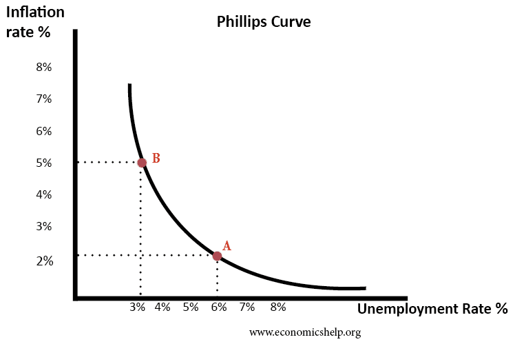
The logic, which builds on our last lesson, is straightforward:

• When an economy is booming, aggregate demand is high.
• To meet this demand, firms hire more workers, so unemployment falls.
• The tight labor market forces firms to offer higher wages to attract and retain employees.
• Firms pass these higher labor costs (and other input costs) on to consumers as higher prices, leading to inflation.

In the 1960s, many economists and policymakers believed this curve represented a stable, long-term trade-off. They viewed it as a "menu of policy options," as described in the Econlib article "Phillips Curve". A government could choose to stimulate the economy to achieve lower unemployment, accepting the "cost" of higher inflation, or it could contract the economy to reduce inflation, accepting the "cost" of higher unemployment.

2. The Long-Run Phillips Curve and the Role of Expectations

This simple trade-off theory came under fire in the 1970s when many countries experienced stagflation—simultaneously high inflation and high unemployment, a combination the original Phillips curve suggested was impossible.

The theoretical challenge came from economists Milton Friedman and Edmund Phelps. They argued that the trade-off was only temporary and existed only as long as workers were surprised by inflation. In the long run, they argued, there is no trade-off.

To understand their argument, we need to introduce two key concepts: inflation expectations and the natural rate of unemployment.

Let's walk through the process described in the reading, using a diagram to illustrate.

1. Initial State (Point on PC1 at Un): The economy is at its natural rate of unemployment (say, 5%) with a stable inflation rate (say, 2%). At this point, expected inflation equals actual inflation.

2. Expansionary Policy (Step 1): The government uses monetary or fiscal policy to boost aggregate demand. Firms hire more workers, and unemployment falls to 4%. This moves the economy along the initial short-run curve (PC1) to a point with higher inflation (3.5%). This trade-off works because the inflation was unexpected. Workers see their nominal wages rise and work more, not immediately realizing that prices have risen even faster, eroding their real wage.

3. Expectations Adjust (Step 2 & 3): Workers are not fooled for long. They begin to expect higher inflation (e.g., 3.5%) and demand higher wage increases to protect their real purchasing power. This increase in expected inflation makes the original trade-off between inflation and unemployment worse. The entire short-run Phillips curve shifts upward (from PC1 to PC2, and eventually to PC3).

4. Long-Run Equilibrium (Point on LRPC): The economy returns to its natural rate of unemployment (5%), but now at a much higher stable rate of inflation (10%). The attempt to permanently keep unemployment below the natural rate has failed, resulting only in accelerating inflation.

This leads to a crucial conclusion:

• The Short-Run Phillips Curve (SRPC) shows a trade-off, but only when inflation expectations are constant.
• The Long-Run Phillips Curve (LRPC) is vertical at the natural rate of unemployment. This means that in the long run, any rate of inflation is compatible with the natural rate of unemployment. There is no trade-off.

The natural rate of unemployment (or NAIRU - Non-Accelerating Inflation Rate of Unemployment) is the unemployment rate that prevails when cyclical unemployment is zero and the inflation rate is stable.

3. Shifts of the Phillips Curve vs. Movements Along It

For the CFA exam, it is vital to distinguish between factors that cause a movement along the SRPC and factors that cause the entire curve to shift.

Movements Along the SRPC

A movement along a stationary SRPC is caused by a change in aggregate demand (AD).

• An increase in AD (e.g., from expansionary fiscal policy) leads to higher output and lower unemployment, moving the economy up and to the left along the SRPC to a point with higher inflation.
• A decrease in AD (e.g., during a recession) leads to lower output and higher unemployment, moving the economy down and to the right along the SRPC to a point with lower inflation.

Shifts of the SRPC

The SRPC shifts when the inflation-unemployment relationship itself changes. This is primarily caused by:

1. Changes in Inflation Expectations: As we saw above, if people expect higher inflation, the SRPC shifts upward/rightward. If they expect lower inflation, it shifts downward/leftward.
2. Supply Shocks: An adverse supply shock (e.g., a sudden surge in oil prices) increases firms' costs of production. This shifts the short-run aggregate supply (SRAS) curve to the left, causing both higher inflation and higher unemployment (stagflation). This corresponds to an upward/rightward shift of the SRPC. A positive supply shock (e.g., a technological breakthrough that lowers costs) would shift the SRPC downward/leftward.

This next video does an excellent job of connecting the AD/AS model you already know to movements and shifts of the Phillips curve.

To reinforce these critical distinctions, the following reading summarizes the rules and provides answers to common questions.

Conclusion

Today we've unpacked the Phillips curve, a central concept in macroeconomics. We've moved from a simple inverse relationship to a more nuanced model that distinguishes between the short run and the long run, with inflation expectations playing the starring role.

Key Takeaways:

• The Short-Run Phillips Curve (SRPC) shows an inverse trade-off between inflation and unemployment, assuming constant inflation expectations.
• The Long-Run Phillips Curve (LRPC) is vertical at the natural rate of unemployment (NAIRU), indicating no long-run trade-off.
• Attempts to use expansionary policy to hold unemployment below the natural rate will only lead to accelerating inflation as expectations adjust and shift the SRPC upward.
• Demand shocks (changes in AD) cause movements along the SRPC.
• Supply shocks and changes in inflation expectations cause the SRPC to shift.

Preview of the Next Lesson:

Now that we have examined the key relationships and phases of the business cycle, we will take a step back in our next lesson to summarize the major macroeconomic theories of business cycles. We will compare the Keynesian, Monetarist, and Real Business Cycle perspectives on what causes economic fluctuations and what, if anything, policymakers should do about them. This will provide a theoretical framework for everything we have discussed in this module.