Introduction
Welcome to our next lesson. In our last session, we constructed the Aggregate Demand (AD) curve, representing the total spending in an economy at various price levels. We explored its components () and the factors that cause the entire curve to shift.
Now, we need to build the supply side of our short-run model. While the Long-Run Aggregate Supply (LRAS) curve represents the economy's potential output, the Short-Run Aggregate Supply (SRAS) curve describes how much firms are willing and able to produce in the immediate term, as conditions change.
This lesson is dedicated to understanding the SRAS curve. By the end of our session, you will be able to describe the SRAS curve, explain why it slopes upward, and identify the key non-price factors that cause it to shift. This is the final component we need before we can bring our full AD-AS model together to analyze short-run economic fluctuations.
1. The Short-Run Aggregate Supply (SRAS) Curve
The short-run aggregate supply curve shows the relationship between the overall price level and the total quantity of goods and services (real GDP) that firms are willing to produce, holding input prices constant.
As you can see in the graph below, the SRAS curve slopes upward. This indicates a direct or positive relationship between the price level and the quantity of output supplied.
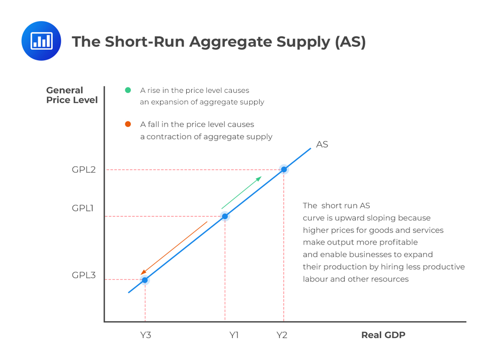
But why does this happen? Why do firms produce more when prices are higher? The key lies in what economists call "sticky" input prices.
To explore this, let's watch the first part of a clear and concise video on this topic.
Short-run Aggregate Supply (SRAS)
This video from Jason Welker defines the short-run in macroeconomics and explains the fundamental reason for the SRAS curve's upward slope.
Please watch the video from the beginning until 06:04. Focus on: The definition of the 'short-run' as the 'fixed wage period'. The concept of 'sticky wages' (and other input costs) and why things like labor contracts and minimum wage laws cause this stickiness. How sticky wages create an incentive for firms to increase output when the price level rises.
The video's central point is that in the short run, many of a firm's costs, especially wages, are fixed or "sticky." When the price level of final goods and services rises, firms receive more revenue for what they sell. However, since their labor costs haven't changed yet, their profit margins increase. This higher potential for profit incentivizes them to increase production.
Conversely, if the price level falls while wages remain fixed, profit margins get squeezed, and firms will cut back on production and employment. This dynamic—where output prices change but input prices lag behind—is what creates the upward-sloping SRAS curve.
2. Shifts in the SRAS Curve
Just like with the demand curve, it's crucial to distinguish between a movement along the SRAS curve and a shift of the entire curve.
- A movement along the curve occurs when the overall price level changes, leading firms to adjust their output levels (as we just discussed).
- A shift of the curve occurs when some factor other than the price level changes the costs of production for many firms in the economy.
A shift to the right (like from SRAS1 to SRAS2 in the graph below) represents an increase in aggregate supply—firms are willing to produce more output at every price level. A shift to the left represents a decrease in aggregate supply.
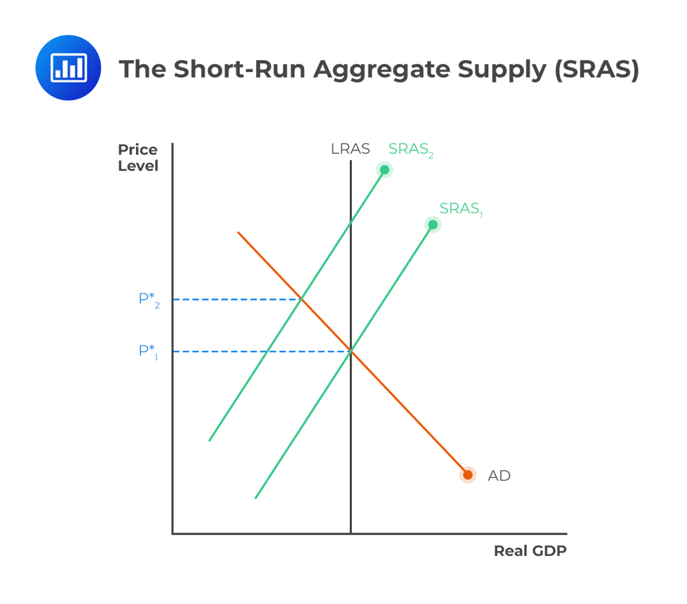
The factors that shift the SRAS curve are all related to the costs of production. Let's get a comprehensive, CFA-focused list of these shifters.
Economics - Learning Module 3 - Aggregate Output, Prices, and Economic Growth
This pre-reading document from Edge Designations, a CFA prep provider, provides a detailed breakdown of the factors that shift the SRAS curve. This text is structured in a way that aligns well with the CFA curriculum.
Please read the section titled 'Factors that change the cost of production or expected profit margins will cause the SRAS curve to shift' (on page 26). Focus on understanding how each of the following affects a firm's costs and thus shifts the SRAS curve: Changes in nominal wages Input prices (like oil, steel, etc.) Expectations about future prices Business taxes and subsidies Exchange rates Supply shocks
To summarize and organize the key shifters from the reading:
| Shifter | Effect on Production Costs | Direction of SRAS Shift |
|---|---|---|
| Increase in Nominal Wages | Increases Costs | Left (Decrease) |
| Decrease in Input Prices (e.g., oil) | Decreases Costs | Right (Increase) |
| Increase in Productivity / Technology | Decreases Costs per unit | Right (Increase) |
| Increase in Expected Future Prices | Increases Current Costs (e.g., wage demands) | Left (Decrease) |
| Increase in Business Taxes | Increases Costs | Left (Decrease) |
| Increase in Business Subsidies | Decreases Costs | Right (Increase) |
| Appreciation of Domestic Currency | Decreases cost of imported inputs | Right (Increase) |
A particularly important factor mentioned in the reading is a supply shock. This is a sudden, often unexpected event that dramatically changes the cost of production for many firms. A classic example is a sharp rise in oil prices, which would be a negative supply shock, increasing costs and shifting the SRAS curve to the left. A new technological breakthrough that boosts productivity would be a positive supply shock.
3. Practice Scenarios
You've mentioned that solving problems helps with retention. The best way to master these shifters is to apply them. Let's work through a few scenarios.
Aggregate Supply- Macro Topics 3.3 and 3.4
This video from Jacob Clifford presents five quick-fire scenarios. It's an excellent way to test your understanding in a format similar to exam questions.
Watch the video from 04:06 to 05:16. For each of the five scenarios presented, pause the video and decide for yourself whether the SRAS curve will increase or decrease and what the shifter is. Then, play the video to check your reasoning against the explanation.
How did you do? Let's review the logic:
- Increase in nominal wages: This directly increases labor costs, shifting SRAS left.
- More physical capital (factories, tools): This increases the economy's productive capacity, shifting SRAS right.
- Widespread power outages: This is a negative supply shock, reducing the ability to produce and shifting SRAS left.
- Decrease in corporate taxes: This lowers production costs for firms, shifting SRAS right.
- Higher expected future prices: Firms and workers will build this into their decisions today. Workers will demand higher wages, and firms may hold back supply, increasing costs and shifting SRAS left.
Mastering these cause-and-effect relationships is essential for the exam.
Conclusion
In this lesson, we have added the final building block to our short-run macroeconomic model: the Short-Run Aggregate Supply curve.
Key Takeaways:
- The SRAS curve shows a positive relationship between the price level and the quantity of real GDP supplied in the short run.
- It slopes upward primarily because of sticky input prices, especially nominal wages. When output prices rise, but costs don't, firms' profit margins expand, incentivizing them to produce more.
- The SRAS curve shifts in response to changes in the economy-wide costs of production.
- Key shifters that decrease SRAS (shift left) include increases in nominal wages, input prices, or business taxes.
- Key shifters that increase SRAS (shift right) include decreases in those costs, or an increase in productivity, technology, or business subsidies.
Preview of the Next Lesson:
We have now independently analyzed the three key curves of our model: Aggregate Demand (AD), Long-Run Aggregate Supply (LRAS), and Short-Run Aggregate Supply (SRAS). In our next lesson, we will finally bring them all together. We will see how they interact to determine the economy's equilibrium price level and real GDP, and, most importantly, we will analyze how the economy responds to various shocks in both the short run and the long run.