LRAS and Potential GDP

1. What is the "Long Run"?

In macroeconomics, the "long run" isn't a specific period of time like five or ten years. Instead, it's a period long enough for all prices in the economy to fully adjust to economic changes. This includes not just the prices of final goods and services, but also input prices like wages and raw materials.

To get a clear idea of this concept, let's watch a short, intuitive explanation.

The key takeaway is that the sticky wages and prices that defined the short run are no longer a factor. In the long run, labor contracts can be renegotiated, rental agreements expire, and raw material prices adjust. Because all prices are fully flexible, the logic that made the SRAS curve upward-sloping no longer applies.

2. The Vertical LRAS Curve and Potential GDP

So, if a change in the price level doesn't create a profit incentive in the long run, what does the aggregate supply curve look like?

In the long run, an economy's ability to produce goods and services depends on its real resources: its stock of capital, its labor force, its natural resources, and its level of technology. These are not affected by the overall price level.

Therefore, the Long-Run Aggregate Supply (LRAS) curve is a vertical line at the economy's potential GDP (also called full-employment output).

Why is it vertical? Imagine the overall price level doubles. In the long run, workers will demand double the nominal wages to maintain their real purchasing power, and suppliers of raw materials will also double their prices. For a firm, both its revenues and its costs have doubled, leaving its real profit margin unchanged. With no change in real profitability, there is no incentive to alter the level of production. Output remains at the level dictated by the economy's real productive capacity.

From Short Run to Long Run

We can demonstrate this relationship more formally. Recall that the equation for the SRAS curve can be expressed as:

$Y=Y^{\ast }+a(P-P_e)$

Where:

• $Y$ is the actual output.
• $Y^{\ast }$ is the potential output (or natural level of production).
• $P$ is the actual price level.
• $P_e$ is the expected price level.
• $a$ is a coefficient representing the responsiveness of output to price surprises.

In the short run, actual prices can differ from expected prices ($P\ne P_e$), causing output to deviate from potential. In the long run, however, expectations adjust and catch up to reality, so $P=P_e$. When this happens, the term $(P-P_e)$ becomes zero.

The SRAS equation simplifies to:
$Y=Y^{\ast }$
This is the equation for the LRAS curve. It states that in the long run, output ($Y$) equals potential output ($Y^{\ast }$), regardless of the price level. This is why the LRAS curve is a vertical line.

The following resource provides a concise summary of this logic.

3. Shifts in the LRAS Curve: The Sources of Economic Growth

If the LRAS curve represents the economy's potential output, a shift in the LRAS curve represents a change in that potential. A rightward shift signifies economic growth, while a leftward shift signifies economic contraction.

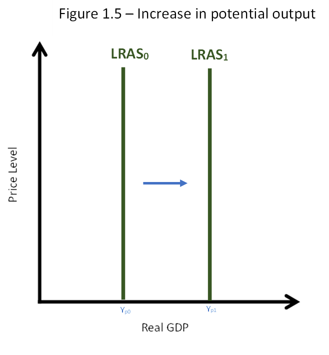
What causes this potential to change? The factors that shift the LRAS are the fundamental drivers of economic growth. Let's watch a video that details these sources from a CFA curriculum perspective.

As the video and supporting texts explain, the key factors that increase potential GDP and shift the LRAS curve to the right are:

• Increase in the supply of labor: A larger workforce means more potential output. This can come from population growth, a higher labor force participation rate, or net immigration.
• Increase in human capital: This refers to the quality of the labor force. Better education, training, and skills make workers more productive.
• Increase in the stock of physical capital: More factories, machinery, tools, and infrastructure enhance the economy's productive capacity.
• Advancements in technology: This is often the most important driver. Technology, or Total Factor Productivity (TFP), refers to the efficiency with which we combine labor and capital. It includes everything from new inventions to better management processes.
• Increase in natural resources: Discovering new deposits of oil or minerals can also increase potential output.

4. Applying the Concepts: Quantifying Growth

For a financial analyst, simply listing the sources of growth is not enough. The CFA curriculum requires you to be familiar with how this growth is measured. The video introduced two key formulas for this.

1. The Growth Accounting Equation

This equation, derived from the Solow growth model, deconstructs the growth of potential GDP into its component parts:

$\Delta Y/Y=\Delta A/A+w_L(\Delta L/L)+w_C(\Delta K/K)$

Where:

• $\Delta Y/Y$ = Growth rate of potential GDP
• $\Delta A/A$ = Growth rate of Total Factor Productivity (technology)
• $\Delta L/L$ = Growth rate of the labor force
• $\Delta K/K$ = Growth rate of the capital stock
• $w_L$ and $w_C$ are the shares of national income paid to labor and capital, respectively (and $w_L+w_C=1$).

Example: Suppose TFP growth is 1%, the labor force grows by 1.5%, and the capital stock grows by 3%. The share of income going to labor is 0.7, and to capital is 0.3.
Potential GDP growth would be:
1% + 0.7(1.5%) + 0.3(3%) = 1% + 1.05% + 0.9% = 2.95%

This tells us how much each factor is contributing to overall economic growth.

2. Estimating Sustainable Growth

Since measuring capital stock and TFP can be difficult, analysts often use a simpler, powerful approximation:

$\text{Potential Growth Rate}\approx \text{Long-term growth of labor force}+\text{Long-term growth of labor productivity}$

This formula is intuitive. The economy can grow for two reasons: you have more workers (growth of labor force), or your existing workers become more productive (growth of labor productivity). As an analyst, you can estimate long-term sustainable GDP growth by forecasting population trends and productivity trends.

Conclusion

This lesson has established the long-run anchor for our macroeconomic model. We've moved beyond short-term fluctuations to understand the economy's underlying productive potential.

Key Takeaways:

• The Long-Run Aggregate Supply (LRAS) curve is vertical because in the long run, all prices are flexible, and output is determined by real factors, not the price level.
• The LRAS curve is located at the level of potential GDP, which is the maximum sustainable output an economy can produce at full employment.
• A shift in the LRAS curve represents economic growth (or contraction).
• The primary sources of economic growth that shift LRAS to the right are increases in the supply of labor and capital, improvements in human capital (quality of labor), and advancements in technology (TFP).
• The growth accounting equation and the labor productivity growth formula are key tools for quantifying and analyzing the sources of potential GDP growth.

Preview of the Next Lesson:

We now have all three of our core curves: the downward-sloping AD curve, the upward-sloping SRAS curve, and the vertical LRAS curve. In our next lesson, we will finally bring them all together in a single model. We will identify short-run and long-run macroeconomic equilibrium and, most importantly, analyze how the economy behaves when it's pushed away from that long-run equilibrium, creating what are known as inflationary and recessionary gaps.