Introduction
Welcome back! In our last lesson, we established the fundamental drivers of long-run economic growth by introducing the production function, , and the growth accounting equation. We saw that an economy's output grows through increases in its inputs—capital and labor—and, most importantly for sustained growth, through improvements in technology and efficiency (Total Factor Productivity).
Today's lesson builds directly on that foundation. We will formally define the concept of an economy's maximum productive capacity, which we call potential GDP, and explore what determines its growth rate, known as the sustainable rate of economic growth. Understanding these concepts is essential for any financial analyst, as they represent the long-term trend around which short-term economic activity fluctuates.
By the end of this lesson, you will be able to explain the concepts of potential GDP and sustainable growth, bridging the gap between the long-run sources of growth and the macroeconomic models we will build next.
1. Defining Potential GDP
What is an economy's "potential"? It's not the absolute maximum it could produce in a short burst, but rather the level of output it can sustain over the long term without creating economic imbalances, like accelerating inflation.
To get an intuitive feel for this, let's watch a short video from the Atlanta Fed.
The Fed Explains Real Versus Potential GDP
This video, 'The Fed Explains Real Versus Potential GDP', uses a simple analogy to explain what potential GDP represents and why it's a crucial benchmark for policymakers.
Watch the video from 01:01 to 03:30. Pay close attention to how it distinguishes between an individual's potential output and their maximum possible output, and how this idea extends to the national economy.
As the video explains, Potential GDP is the maximum amount of real output an economy can produce over a period of time with the full, sustainable employment of its available resources (capital, labor, and technology). It's the level of output achieved when the economy is operating at the "natural" rate of unemployment.
Key Connections:
- Production Function: In the context of our last lesson, potential GDP is the level of output () generated when the labor input () is at its "full-employment" level.

- AD-AS Model: In the Aggregate Demand/Aggregate Supply model, which we are building towards, potential GDP is represented by the Long-Run Aggregate Supply (LRAS) curve. Because potential GDP depends on the real factors of production (capital, labor, technology) and not the price level, the LRAS curve is vertical.
An economy's actual real GDP can, and often does, differ from its potential GDP in the short run.
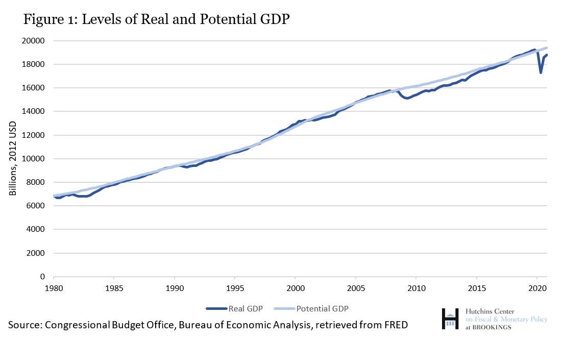
It's crucial to distinguish between a short-term boost in real GDP and a genuine increase in the economy's potential.
Level 1 CFA Economics: Aggregate Output Prices and Economic Output-Lecture 6
Let's watch a segment of the IFT video you've seen before. It does an excellent job of illustrating the difference between a movement to a new short-run equilibrium and a shift of the long-run potential.
Watch the segment from 01:39 to 03:58. Focus on how the AD-AS graph is used to show why an increase in potential GDP (a shift in the LRAS curve) is more significant for long-term investors than a short-term increase in real GDP (caused by a shift in the AD curve).
2. The Sustainable Rate of Growth
If potential GDP represents the economy's long-run productive capacity, then the rate at which this capacity grows is the sustainable rate of economic growth. It's the speed limit for the economy—the rate at which it can grow year after year without generating inflationary pressures.
The sources of this growth are exactly what we discussed in the last lesson: growth in the supply and quality of labor, growth in the capital stock, and advances in technology. The growth accounting equation we studied provides the detailed theoretical breakdown.
However, for practical estimation purposes, especially since Total Factor Productivity (TFP) is difficult to measure directly, analysts often use a more straightforward approach based on labor.
To understand this practical approach, please read the following sections from the CFA pre-reading notes.
PRE-READING Economics - Learning Module 3
This reading from Edge Designations provides a concise and examinable overview of how sustainable growth is defined and measured. It links the concepts of the production function, potential GDP, and labor productivity.
Please read the following three sections in the PDF: 'The Production Function and Potential GDP' (page 33-34): Review the definition of the production function and the growth accounting equation. 'Sources of economic growth' (page 35): Note the definition of the sustainable growth rate. 'Measures of Sustainable Growth' (page 37-38): This is the core section. Focus on how potential GDP can be described in terms of labor and productivity, and memorize the final formula for the potential growth rate.
As the reading explains, we can express potential GDP as:
When we convert this relationship into growth rates, we arrive at a key formula for the CFA exam:
This formula is powerful because it breaks down sustainable growth into two observable components:
- Growth of Labor Force: How many more people (or hours) are available to work.
- Growth of Labor Productivity: How much more each worker (or hour) can produce. This component is where the effects of capital deepening (more capital per worker) and technology (TFP) are captured.
3. Practice Question
Let's apply this with a typical CFA-style question.
An analyst gathers the following long-term forecasts for a developed economy:
- Growth rate of the labor force: 0.5%
- Growth rate of capital stock: 3.0%
- Share of labor in national income (WL): 0.6
- Share of capital in national income (WC): 0.4
- Long-term labor productivity growth rate: 1.5%
Based on this data, the sustainable rate of economic growth is closest to:
A. 2.0%
B. 2.7%
C. 3.5%
Click to see the solution
The correct answer is A.
The most direct way to answer this question is to use the formula for the potential growth rate based on labor:
You might be tempted to use the growth accounting equation with the capital growth data. Let's see what that would give us. We would need the growth in Total Factor Productivity (TFP). The growth accounting equation is:
Growth in Potential GDP = Growth in TFP + W_L(Growth in Labor) + W_C(Growth in Capital)
We aren't given the TFP growth rate. The question provides the labor productivity growth rate, which already accounts for the contributions of capital deepening and TFP. Therefore, simply summing the labor force growth and labor productivity growth is the correct and most direct method.
Conclusion
In this lesson, we put a formal structure around the concept of an economy's long-term productive capacity. We defined potential GDP and saw how it's represented graphically by the LRAS curve, serving as the economy's sustainable, non-inflationary output level.
Key Takeaways:
- Potential GDP is the level of real GDP an economy can produce at full employment without triggering rising inflation. It is determined by real factors of production: labor, capital, and technology.
- Actual real GDP can deviate from potential, creating inflationary gaps (actual > potential) or recessionary gaps (actual < potential).
- Sustainable growth is the growth rate of potential GDP.
- A practical formula for estimating the sustainable growth rate is to sum the long-term growth rates of the labor force and labor productivity.
Preview of the Next Lesson:
We have now thoroughly examined the supply side of the economy in the long run (LRAS). To understand short-run economic fluctuations, we need to introduce the demand side. In our next lesson, we will describe the components of aggregate demand (AD) and explain the factors that cause the AD curve to shift. This will be the next major step in building the complete AD-AS model.