Monetary and Fiscal Policy: Coordination and Conflict

1. A Framework for Policy Interaction

To understand how these policies interact, we first need to recall their basic stances:

• Fiscal Policy (Government-led):
  • Expansionary (Easy): Aims to increase aggregate demand (AD) through higher government spending (G) or lower taxes (T).
  • Contractionary (Tight): Aims to decrease AD through lower G or higher T.
• Monetary Policy (Central Bank-led):
  • Expansionary (Easy): Aims to increase AD by lowering policy interest rates, making borrowing cheaper.
  • Contractionary (Tight): Aims to decrease AD by raising policy interest rates, making borrowing more expensive.

The overall impact on the economy depends on which stance each authority takes. We can visualize the four possible combinations in a simple 2x2 matrix.

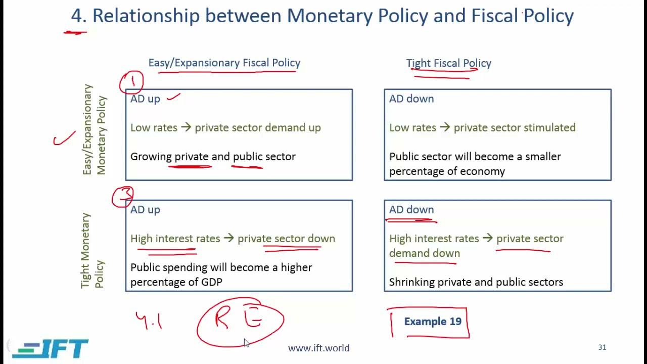
As you can see, two quadrants represent conflicting policies, where the government and central bank are pulling in opposite directions. The other two represent reinforcing policies, where they work in coordination. Let's explore each scenario in detail.

2. The Four Scenarios of Policy Interaction

The best way to understand these interactions is to examine the outcome of each of the four possible policy mixes. The following reading provides a concise explanation of each scenario.

Now that you have an overview from the reading, let's solidify this understanding by watching a short video explanation and breaking down the effects for each case.

Let's synthesize the information from both resources.

Case 1: Easy Fiscal Policy / Tight Monetary Policy

• The Scenario: The government is trying to stimulate the economy (e.g., by increasing infrastructure spending), but the central bank is trying to cool it down (by raising interest rates), perhaps due to inflation concerns.
• Impact:
  • Aggregate Demand: The effect is ambiguous. Fiscal stimulus pushes AD up, while monetary tightening pushes it down. The net effect depends on the relative strength of the two policies.
  • Interest Rates: Will be high. The government's borrowing to fund its spending increases demand for loanable funds, while the central bank is actively restricting the money supply.
  • Economic Mix: The high interest rates "crowd out" private investment and spending. The public sector's share of the economy grows, while the private sector's share shrinks.

Case 2: Tight Fiscal Policy / Easy Monetary Policy

• The Scenario: The government is practicing fiscal discipline (e.g., cutting spending to reduce a deficit), while the central bank is lowering interest rates to support growth.
• Impact:
  • Aggregate Demand: The effect is again ambiguous, depending on which policy is stronger.
  • Interest Rates: Will be low. The government is borrowing less (or not at all), and the central bank is making credit cheap.
  • Economic Mix: This environment is highly favorable for the private sector. Low interest rates encourage business investment and consumer borrowing for big-ticket items. The private sector's share of the economy grows, while the public sector's share shrinks. This mix is often considered ideal for fostering long-term private-sector-led growth.

Case 3: Easy Fiscal Policy / Easy Monetary Policy

• The Scenario: Both the government and the central bank are trying to stimulate the economy. This is a coordinated expansionary effort, often seen during a deep recession.
• Impact:
  • Aggregate Demand: A strong, unambiguous increase. Both policies are pushing in the same direction.
  • Interest Rates: The effect is ambiguous. Fiscal stimulus puts upward pressure on rates (due to borrowing), while monetary easing puts downward pressure. The final outcome depends on which effect is larger.
  • Economic Mix: Both the public sector (through government spending) and the private sector (through low interest rates) are stimulated to expand. This policy mix carries a significant risk of causing high inflation.

Case 4: Tight Fiscal Policy / Tight Monetary Policy

• The Scenario: Both the government and the central bank are trying to slow the economy down. This is a coordinated contractionary effort, used to fight severe inflation.
• Impact:
  • Aggregate Demand: A strong, unambiguous decrease.
  • Interest Rates: Will be high. The government is reducing its pressure on financial markets, but the central bank is aggressively tightening credit.
  • Economic Mix: Aggregate demand from both the public sector (due to spending cuts) and the private sector (due to high interest rates) will fall.

3. Practice Question

Let's apply these concepts with a practice question that touches on a nuance of policy effectiveness.

The correct answer is A. Direct government spending on goods and services (G) is a direct component of aggregate demand. In contrast, tax cuts and transfer benefits only affect aggregate demand if the recipients choose to spend the extra money, and some of it may be saved. Therefore, direct government expenditure generally has the largest and most immediate impact on GDP.

Conclusion

In this lesson, we have explored the critical interactions between monetary and fiscal policy. You are now equipped to analyze how their coordination—or conflict—shapes macroeconomic outcomes.

Key Takeaways:

• The overall impact of macroeconomic policy depends on the combined stance of fiscal and monetary authorities.
• Easy Fiscal / Tight Monetary: Leads to high interest rates and a larger public sector at the expense of the private sector.
• Tight Fiscal / Easy Monetary: Leads to low interest rates and encourages private sector growth.
• Easy Fiscal / Easy Monetary: Provides the strongest stimulus to aggregate demand but risks high inflation.
• Tight Fiscal / Tight Monetary: Exerts the strongest brake on aggregate demand and is used to fight high inflation.
• Understanding this policy mix is crucial for interpreting government and central bank actions and predicting their economic consequences.

Preview of the Next Lesson:

This lesson concludes our module on Macroeconomic Management. We have covered the tools, objectives, and interactions of both monetary and fiscal policy.

We will now shift our focus from a single country's domestic economy to the global economic system. In our next lesson, we will begin the International Trade and Capital Flows module by addressing the learning outcome: Explain absolute and comparative advantage and use opportunity costs to determine trade patterns. We will explore the fundamental reasons why countries trade with one another.