Predicting Narrow, Wide, and Shuffle Dependencies in PySpark Transformations

Think about where each row needs to go

Suppose an orders DataFrame is spread across several partitions. A filter such as amount > 100 can inspect each row where it already resides. Every partition can produce its own filtered output independently. This is a narrow dependency: Spark does not need to redistribute rows among partitions to perform the filter.

Now suppose you need total sales by region. Orders for one region may be scattered across many input partitions. Spark can calculate partial totals locally, but it must bring those partial totals together by region to finish the aggregation. That redistribution is a shuffle, and it creates a wide dependency between the work before and after it.

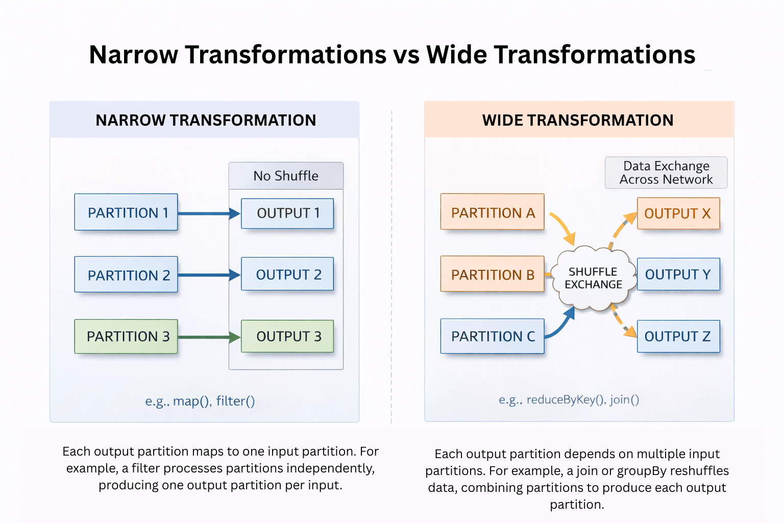
The distinction is about dependencies between partitions, not how many PySpark methods appear in your code. A narrow operation may still be expensive if it processes a great deal of data; a wide operation may be essential to produce the correct answer. The useful prediction is whether an operation needs a shuffle—and therefore usually a boundary between stages—not whether it is universally “good” or “bad.”

There is also a subtlety in the diagram: a narrow operation can combine several whole input partitions into one output partition without redistributing their individual rows by key. coalesce commonly does this. What makes an aggregation wide is that rows or partial results from an input partition may need to be routed to different destination partitions according to their keys.

What a shuffle actually costs

The official Spark RDD Programming Guide explains shuffling using key-based aggregation. Its examples use RDD methods rather than DataFrame methods, but the partition-level problem is the same one Spark must solve for a DataFrame groupBy.

A shuffle can require serialization, sorting or organizing intermediate data, disk I/O, and data transfer. Some transfer can remain on the same machine; it is more precise to say that a shuffle can involve network traffic than that every shuffled row necessarily crosses the network. Conversely, data moving over a network does not always mean a shuffle: a broadcast join distributes a small input without repartitioning the larger input by the join key.

Watch a short visual explanation, followed by an example of where redistribution appears in a query plan.

Predicting common DataFrame transformations

Start with a simple question: Could a task produce its output using only the rows already available in its input partition? If so, expect a narrow dependency. If correct results require rows with the same key—or rows destined for the same output range—to be gathered from across partitions, expect a shuffle unless the inputs already have a suitable distribution.

For example, these operations are ordinarily narrow:

from pyspark.sql import functions as F

filtered = orders.filter(F.col("amount") > 100)
projected = filtered.select("region", "amount")
adjusted = projected.withColumn("taxed_amount", F.col("amount") * 1.1)

Filtering, selecting columns, and calculating a row-level expression do not require information from other rows. drop, withColumnRenamed, and a row-level when(...).otherwise(...) expression follow the same reasoning. A row-expanding operation such as explode can emit several rows for one input row, but those rows can still be produced locally. More output rows does not, by itself, mean a wide dependency.

Here is a practical prediction guide. “Usually” matters: Spark plans the whole query and can remove redundant work or use an existing data distribution.

A few contrasts prevent common interview mistakes:

• unionByName is not the same as deduplication. The union itself can append partitions narrowly; adding distinct() afterward usually introduces a shuffle.
• sortWithinPartitions("amount") sorts inside each existing partition. It does not promise a global ordering and does not itself require a repartitioning shuffle. orderBy("amount") requests a global order, so a shuffle is usually needed.
• orders.count() is an action that requests a total. orders.groupBy("region").count() describes a grouped DataFrame transformation. The names look similar, but the latter must typically bring partial counts together by region when an action eventually runs it.
• Changing the number of partitions does not determine the dependency type. coalesce(4) can reduce partitions without shuffling; repartition(4) generally redistributes rows even if the input already has four partitions.

These predictions concern the operation itself. A DataFrame may already contain a shuffle earlier in its lineage; calling filter on that DataFrame does not make the filter wide.

Why a join needs a qualified answer

A join is the best test of whether you are reasoning about data movement rather than memorizing method names. Consider joining large orders and customer DataFrames on customer_id:

joined = orders.join(customers, on="customer_id")

For a shuffle-based join, matching keys must reach compatible partitions. If the inputs are not already suitably distributed, Spark may shuffle one or both sides. A plan might therefore show Exchange operators before the join.

But “every join shuffles both tables” is incorrect. If one input is small enough and Spark chooses a broadcast join, it can distribute that input to executor tasks while the larger input remains in its existing partitions. Broadcasting has a transfer cost, but it is not a shuffle of the larger input by join key. Spark can also avoid a redundant shuffle when an input’s existing distribution satisfies the join’s requirements. Which strategy wins depends on the data, statistics, configuration, and optimizer decisions; we will examine those choices later in the course.

The same qualification applies to aggregation. groupBy("region").agg(...) typically needs a shuffle, but Spark need not add another redistribution if the required distribution has already been established and preserved. Predict from the required distribution, then verify the chosen plan.

Window functions offer a brief preview of this principle. A calculation partitioned by customer_id needs each customer’s relevant rows together, and an ordered window needs those rows sorted appropriately. That often entails a shuffle and a sort; the window method name alone does not tell you whether the input already meets those requirements. We will implement windows in a later lesson.

Check the prediction with explain

Return to the regional sales example, now with a global sort:

regional_sales = (
    orders
    .filter(F.col("amount") > 100)
    .select("region", "amount")
    .groupBy("region")
    .agg(F.sum("amount").alias("sales"))
    .orderBy(F.col("sales").desc())
)

regional_sales.explain("formatted")

Read this plan by asking where Spark must change the distribution of the data. The filter and projection can generally run with the scan. For the aggregation, look for an Exchange that distributes partial results by region. For the global orderBy, you may see another Exchange associated with range partitioning, along with sorting work. The exact output depends on the optimizer and runtime settings; do not infer that there must be exactly two exchanges merely because two methods look wide.

An Exchange describing hash, range, or round-robin partitioning is the physical-plan clue for a shuffle. A BroadcastExchange is different: it prepares an input for broadcast, rather than repartitioning rows across shuffle partitions. A Sort operator on its own means sorting work, not necessarily a separate shuffle.

This connects directly to the previous lesson. Work that can be performed within existing partitions may be pipelined in a stage. A shuffle dependency separates work into stages whose later tasks consume shuffled output. explain lets you inspect the planned data movement before an action processes the full DataFrame; the Spark UI can then show what ran.

For an interview, a reliable answer has three parts: name the distribution the result requires, compare it with the input’s distribution, and identify the likely exchange or exception. For example: “Filtering is partition-local. Grouping by region usually shuffles partial results by region. A subsequent global sort may need another redistribution; I would confirm the actual exchanges in the physical plan.”

Conclusion

Narrow dependencies let Spark process data using existing partitions without a repartitioning shuffle. Wide dependencies arise when results require data to be redistributed across partitions, as commonly happens with grouped aggregation, deduplication, global sorting, and shuffle-based joins. coalesce versus repartition, and shuffle joins versus broadcast joins, show why method names are useful clues but not complete answers.

Next, you will put several of these transformations to work in PySpark: filtering and projecting columns, building aggregations, and expressing conditional business rules.