Vector Norms and Angles

Introduction

In our last lesson, we established a formal algebraic understanding of vectors and the dot product, defining it as the sum of component-wise products, $u \cdot v = \sum u_{i} v_{i}$ . We ended with a preview of its geometric meaning and its power in determining orthogonality. Today, we complete that picture.

This lesson bridges the gap between the algebra of vectors and their geometry. You will learn how to measure a vector's length, or norm, and then use that concept along with the dot product to find the precise angle between any two vectors. We will explore two of the most important norms in machine learning, the L1 and L2 norms, and understand their distinct properties. Fulfilling the promise from last time, you will see how the algebraic dot product beautifully encodes geometric information about length and angle, a cornerstone of many machine learning algorithms.

Measuring Vector Length: Norms

The "length" or "magnitude" of a vector is formalized by a concept called a norm. While there are many ways to define a norm, we will focus on the two most prevalent in machine learning: the L2 norm and the L1 norm.

The L2 Norm: Euclidean Length

The most intuitive way to think about a vector's length is the one you are likely familiar with from geometry: the straight-line distance from the origin to the point the vector represents. This is calculated using the Pythagorean theorem, extended to $n$ dimensions. This is formally called the L2 norm or Euclidean norm.

For a vector $v = (v_{1}, v_{2}, \dots, v_{n})$ , its L2 norm, denoted $∣∣ v ∣ ∣_{2}$ , is:

∣∣ v ∣ ∣_{2} = v_{1}^{2} + v_{2}^{2} + \dots + v_{n}^{2} = i = 1 \sum n v_{i}^{2}

Notice the connection to the dot product from our previous lesson. The term inside the square root is simply the dot product of the vector with itself:

∣∣ v ∣ ∣_{2}^{2} = v \cdot v

This relationship, $∣∣ v ∣ ∣_{2} = v \cdot v$ , is a crucial identity that links the algebraic dot product to the geometric concept of length.

The L1 Norm: Manhattan Distance

Another important way to measure vector magnitude is the L1 norm, also known as the "Manhattan distance" or "taxicab norm". Instead of the "as the crow flies" Euclidean distance, the L1 norm measures the distance by summing the absolute values of the components, as if you were constrained to travel along a grid.

For the same vector $v$ , its L1 norm, denoted $∣∣ v ∣ ∣_{1}$ , is:

∣∣ v ∣ ∣_{1} = ∣ v_{1} ∣ + ∣ v_{2} ∣ + \dots + ∣ v_{n} ∣ = i = 1 \sum n ∣ v_{i} ∣

The following video provides an excellent explanation of both the L1 and L2 norms, their geometric interpretations, and how they generalize to higher dimensions.

Vector Norms

This video from ritvikmath provides a clear, comparative introduction to the L1 and L2 vector norms.

First, watch the definition of the L2 norm and its geometric interpretation as Cartesian distance: the introduction. Next, watch the definition of the L1 norm and its "Manhattan distance" interpretation: the L1 norm. Pay close attention to the visual explanation of what the set of all vectors with a constant norm looks like for L2 (a circle) versus L1 (a diamond): the geometric shapes. This difference is fundamental to their use in machine learning. Finally, see how these definitions are generalized to arbitrary dimensions: the generalization.

The sharp "corners" of the L1 norm's diamond shape, as opposed to the smooth circle of the L2 norm, is not just a geometric curiosity. In optimization problems, this property makes the L1 norm tend to produce sparse solutions (i.e., solutions with many zero components). This is used in techniques like LASSO regression for feature selection, a topic we may touch on much later in your learning path. The L2 norm, in contrast, is foundational for algorithms where smooth, continuous notions of distance are paramount.

From Norms and Dot Products to Angles

Now that we have a formal definition for a vector's length (its L2 norm), we can fully unpack the geometric definition of the dot product.

Recall the two vectors $a$ and $b$ in the image below. The dot product relates their algebraic components to their geometric properties.

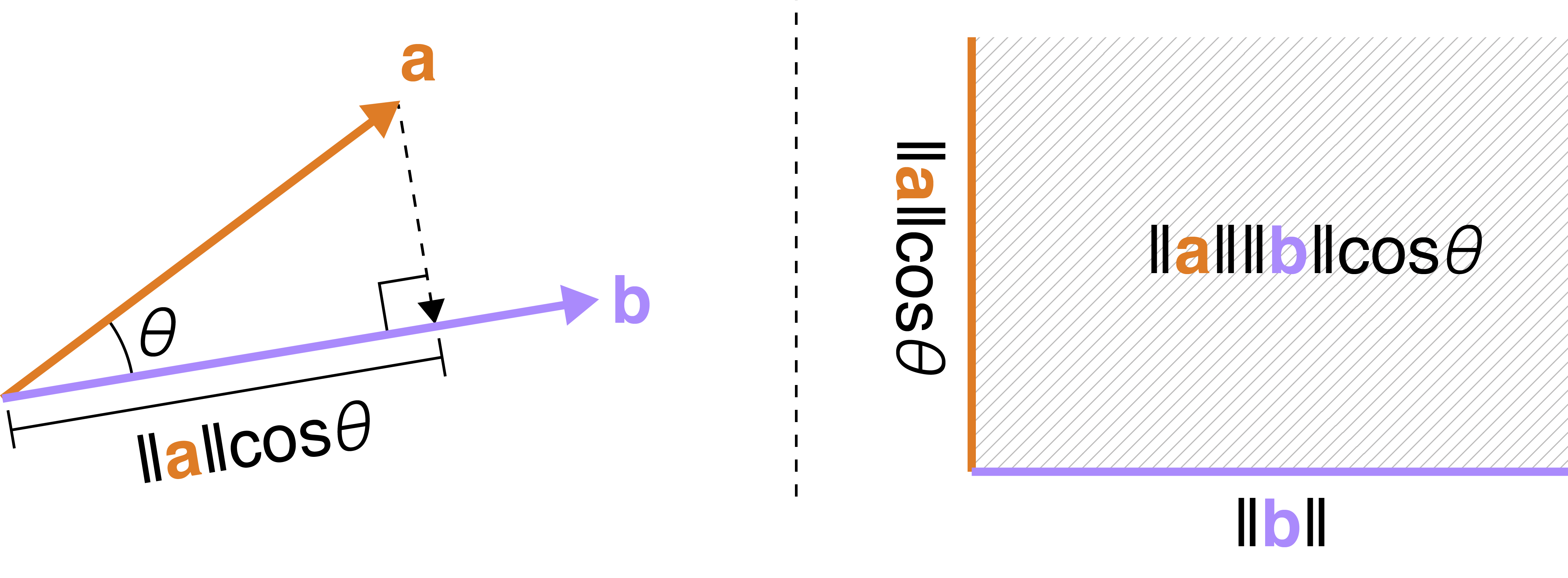
The geometric relationship between two vectors $\mathbf{a}$ and $\mathbf{b}$. The dot product is the product of their lengths (L2 norms) and the cosine of the angle $\theta$ between them. The term $||\mathbf{a}|| \cos\theta$ represents the scalar projection of $\mathbf{a}$ onto $\mathbf{b}$.

The relationship is given by the theorem:

a \cdot b = ∣∣ a ∣ ∣_{2} ∣∣ b ∣ ∣_{2} cos θ

This equation is remarkable because it states that the algebraic operation on the left (sum of products of components) is equal to the geometric operation on the right (product of lengths and the cosine of the angle). Since you value rigor, it's essential to see why this is true. The following reading provides a formal proof based on the Law of Cosines.

Dot Product - Calculus II

This resource from Paul's Online Math Notes proves the geometric formula for the dot product and shows how to use it.

Please read the section that begins with the theorem relating the dot product to the angle. Focus on: The statement of the Theorem: the main formula. The subsequent Proof: This proof uses the Law of Cosines and the property ||\mathbf{v}||^2 = \mathbf{v} \cdot \mathbf{v} to establish the equivalence. Working through this is an excellent exercise in connecting these concepts. The worked Example 2: This shows how to apply the formula to find the angle between two specific vectors.

By rearranging the formula, we get a direct way to compute the angle between two vectors:

cos θ = \frac{a \cdot b}{∣∣ a ∣ ∣ _{2} ∣∣ b ∣ ∣ _{2}}

θ = arccos (\frac{a \cdot b}{∣∣ a ∣ ∣ _{2} ∣∣ b ∣ ∣ _{2}})

This formula is the computational engine for finding angles in any dimension. To see it in action, let's watch a clear, step-by-step calculation.

Linear Algebra 5.1 Length and Dot Product in Rn

In this video, Kimberly Brehm derives and applies the formula for the angle between two vectors.

First, watch the brief derivation that starts from the Law of Cosines and arrives at the final formula for \cos \theta: the derivation. This provides a slightly different but equivalent path to the one in the text you just read. Then, watch the worked-out example of calculating the angle between two 4-dimensional vectors: the example calculation. Note how the process is exactly the same as in 2D or 3D: compute the dot product and the two norms, then find the arccosine of their ratio.

Application: Cosine Similarity

The term $cos θ$ is so useful in machine learning that it has its own name: cosine similarity. When vectors represent objects like words or documents (as they do in LLMs), cosine similarity measures how alike they are in terms of direction, ignoring their magnitude.

A cosine similarity of 1 means $θ = 0^{\circ}$ . The vectors point in the same direction. They are maximally similar.
A cosine similarity of 0 means $θ = 9 0^{\circ}$ . The vectors are orthogonal. They have no similarity in this context.
A cosine similarity of -1 means $θ = 18 0^{\circ}$ . The vectors point in opposite directions. They are maximally dissimilar.

For example, in a well-trained word embedding model, the vectors for "cat" and "kitten" would have a cosine similarity close to 1, while the vectors for "cat" and "skyscraper" would have a cosine similarity close to 0. This is a fundamental tool for reasoning in high-dimensional spaces.

Conclusion

In this lesson, we have added essential geometric tools to our linear algebra toolkit. We have seen how the abstract concept of a vector's "length" is made concrete through norms, and we explored the two most important ones for machine learning. Most critically, we connected the algebraic dot product to the geometric concepts of length and angle, culminating in a method to precisely calculate the angle between any two vectors.

Key Takeaways:

A norm is a function that assigns a positive length or size to each vector.
The L2 norm ( $∣∣ v ∣ ∣_{2} = \sum v_{i}^{2}$ ) represents the standard Euclidean length and is equal to $v \cdot v$ .
The L1 norm ( $∣∣ v ∣ ∣_{1} = \sum ∣ v_{i} ∣$ ) represents the "Manhattan" or "taxicab" distance.
The angle $θ$ between two vectors $a$ and $b$ is found using the formula: $θ = arccos (\frac{a \cdot b}{∣∣ a ∣ ∣ _{2} ∣∣ b ∣ ∣ _{2}})$ .
Cosine similarity ( $cos θ$ ) is a vital metric in machine learning for measuring the directional similarity between vectors, independent of their magnitude.

We are now equipped with the fundamental operations and geometric interpretations of vectors. In our next lesson, we will explore how vectors can be combined to form other vectors through linear combinations, and we will introduce the crucial concept of linear independence. This will lay the groundwork for understanding the structure of vector spaces and bases.

Recommended resources