Graphing Functions from Features

Power and Polynomial Functions: The Building Blocks

Let's begin with the most basic type of polynomial: a power function. These are the fundamental units from which more complex polynomials are built.

A power function has the form $f(x)=k{x}^p$, where $k$ and $p$ are real numbers. For our current focus on polynomials, we will primarily consider cases where $p$ is a non-negative integer.

The key to understanding power functions—and, by extension, all polynomials—is their end behavior: what happens to the function's values as $x$ approaches positive or negative infinity ($x\to \infty$ or $x\to -\infty$). This behavior is determined entirely by two things:

1. Whether the power $p$ is even or odd.
2. Whether the coefficient $k$ is positive or negative.

This should sound familiar! The even/odd nature of the exponent directly relates to the even/odd symmetry we discussed in the last lesson. Professor Leonard provides an excellent conceptual overview of this connection.

As you saw in the video, the end behavior of a power function $f(x)=k{x}^p$ (where $p$ is a positive integer) follows four predictable patterns:

• p is even, k > 0: Graph goes up on both ends (e.g., $x^2$). As $x\to \pm \infty$, $f(x)\to \infty$.
• p is even, k < 0: Graph goes down on both ends (e.g., $-x^2$). As $x\to \pm \infty$, $f(x)\to -\infty$.
• p is odd, k > 0: Graph goes down on the left, up on the right (e.g., $x^3$). As $x\to -\infty$, $f(x)\to -\infty$; as $x\to \infty$, $f(x)\to \infty$.
• p is odd, k < 0: Graph goes up on the left, down on the right (e.g., $-x^3$). As $x\to -\infty$, $f(x)\to \infty$; as $x\to \infty$, $f(x)\to -\infty$.

This is the cornerstone for analyzing more complex polynomials. A polynomial function is simply a sum of power functions with non-negative integer exponents.

When sketching a polynomial, the most important term is the leading term, $a_n{x}^n$. This is the power function with the highest exponent, and it single-handedly dictates the polynomial's end behavior. As $x$ becomes very large (positive or negative), the leading term grows much faster than all other terms, dominating the function's behavior.

The following reading formalizes these concepts.

Sketching Polynomials: Zeros and Multiplicity

End behavior gives us the "big picture" of the graph. To fill in the details, we need to find where the graph crosses the axes, particularly the x-axis. These x-intercepts are called the zeros or roots of the polynomial.

To find the zeros, we set $f(x)=0$ and solve for $x$. If the polynomial is factored, this is straightforward. For example, if $f(x)=(x-2)(x+3)$, the zeros are $x=2$ and $x=-3$.

The multiplicity of a zero is the number of times its corresponding factor appears. This tells us how the graph behaves at the x-intercept:

• Multiplicity 1: The graph crosses the x-axis cleanly (like a line).
• Multiplicity 2 (or any even number): The graph touches the x-axis and "bounces" off (like a parabola).
• Multiplicity 3 (or any odd number > 1): The graph crosses the x-axis but flattens out as it does so, creating an "S-curve" shape (like $y=x^3$).

The following video provides an excellent guide to using end behavior, zeros, and multiplicities to sketch a polynomial.

To summarize the process for sketching a polynomial:

1. End Behavior: Find the degree and leading coefficient. Determine if the graph rises or falls on the far left and far right.
2. Intercepts: Find the y-intercept by calculating $f(0)$. Find the x-intercepts (zeros) by setting $f(x)=0$ and solving.
3. Multiplicities: Determine the multiplicity of each zero to know if the graph crosses or bounces at the x-axis.
4. Sketch: Start from one end, draw the graph through the intercepts with the correct behavior, and connect to the other end.

Rational Functions: Ratios and Asymptotes

Now we turn to rational functions, which are functions formed by the ratio of two polynomials: $f(x)=\frac{P(x)}{Q(x)}$.

Their graphs can be more complex than polynomials. The key new features are asymptotes: lines that the graph approaches but typically does not cross.

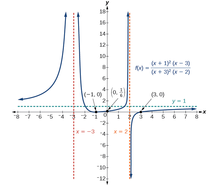
Analyzing a rational function involves a systematic checklist. The following resource provides a comprehensive step-by-step guide.

Let's focus on the most critical features from that guide: asymptotes and intercepts.

1. Vertical Asymptotes and Holes

A vertical asymptote occurs where the function is undefined—that is, where the denominator $Q(x)=0$. However, there's a catch. You must first simplify the fraction. If a factor $(x-c)$ cancels out from both the numerator and denominator, there is a hole in the graph at $x=c$, not a vertical asymptote.

• Vertical Asymptote: Occurs at $x=c$ if $Q(c)=0$ and $P(c)\ne 0$ after simplification.
• Hole: Occurs at $x=c$ if the factor $(x-c)$ can be cancelled from the numerator and denominator.

2. Horizontal Asymptotes

Horizontal asymptotes describe the end behavior of the function. You find them by comparing the degree of the numerator, deg(P), to the degree of the denominator, deg(Q).

• deg(P) < deg(Q): The horizontal asymptote is the x-axis, $y=0$.
• deg(P) = deg(Q): The horizontal asymptote is $y=\frac{\text{leading coefficient of }P}{\text{leading coefficient of }Q}$.
• deg(P) > deg(Q): There is no horizontal asymptote.

3. Slant (Oblique) Asymptotes

In the special case where deg(P) is exactly one more than deg(Q), the graph has a slant asymptote. This is a slanted line that the graph approaches. You find the equation of this line by performing polynomial long division of $P(x)$ by $Q(x)$. The quotient (ignoring the remainder) is the equation of the slant asymptote.

4. Intercepts

• y-intercept: Find $f(0)$.
• x-intercepts: Set the numerator $P(x)=0$ and solve. (These are the zeros of the numerator).

The following resource provides clear explanations and examples for finding each type of asymptote.

By systematically finding the domain, intercepts, holes, and all asymptotes, you can piece together an accurate sketch of any rational function.

Conclusion

In this lesson, we added three major families of functions to your mathematical library: power, polynomial, and rational functions. You learned to deconstruct their formulas to predict their graphical behavior.

Key Takeaways:

• Power Functions ($k{x}^p$): Their end behavior is dictated by the parity (even/odd) of the exponent $p$ and the sign of the coefficient $k$.
• Polynomial Functions: They are sums of power functions. Their end behavior matches that of their leading term. Their local behavior is governed by the zeros (x-intercepts) and their multiplicities, which determine if the graph crosses or bounces at the axis.
• Rational Functions ($P(x)/Q(x)$): Their graphs are characterized by asymptotes.
  • Vertical asymptotes occur where the simplified denominator is zero.
  • Horizontal or slant asymptotes describe the end behavior and are found by comparing the degrees of the numerator and denominator.
  • Holes occur at x-values corresponding to factors that cancel out.

In our next lesson, we will move on to the next learning outcome: Graph complex functions by applying horizontal and vertical shifts, stretches, and reflections to parent functions. The "parent" functions we've studied today—like $x^2$, $x^3$, and $1/x$—will serve as the foundation upon which we will build more intricate graphs using these transformations.