The Derivative as a Limit of Difference Quotients

1. The Tangent and Velocity Problems

Imagine trying to find the slope of a curved line. To calculate a slope, you need two points. But at a specific point on a curve, you only have one. How can we find the slope of the tangent line—the line that just skims the curve at that single point?

Similarly, consider a rocket accelerating into space. Its speed is constantly changing. If you calculate its speed over a 10-second interval, you're only finding its average velocity. How can we determine its instantaneous velocity at the precise moment it passes 1,000 meters in altitude?

Both problems hinge on the same idea: we can start with an approximation using two points and then improve that approximation by moving the points infinitely close together. This process of "getting infinitely close" is exactly what limits are for.

The following video provides an excellent conceptual introduction to this idea using the rocket example. It illustrates how we move from a crude approximation (average velocity) to a precise answer (instantaneous velocity) by shrinking the interval between two points.

2. From Secant Lines to the Tangent Line

As the video demonstrated, we can approximate the slope of the tangent line at a point $P$ by choosing a second point $Q$ on the curve and calculating the slope of the line that passes through both. This is called a secant line.

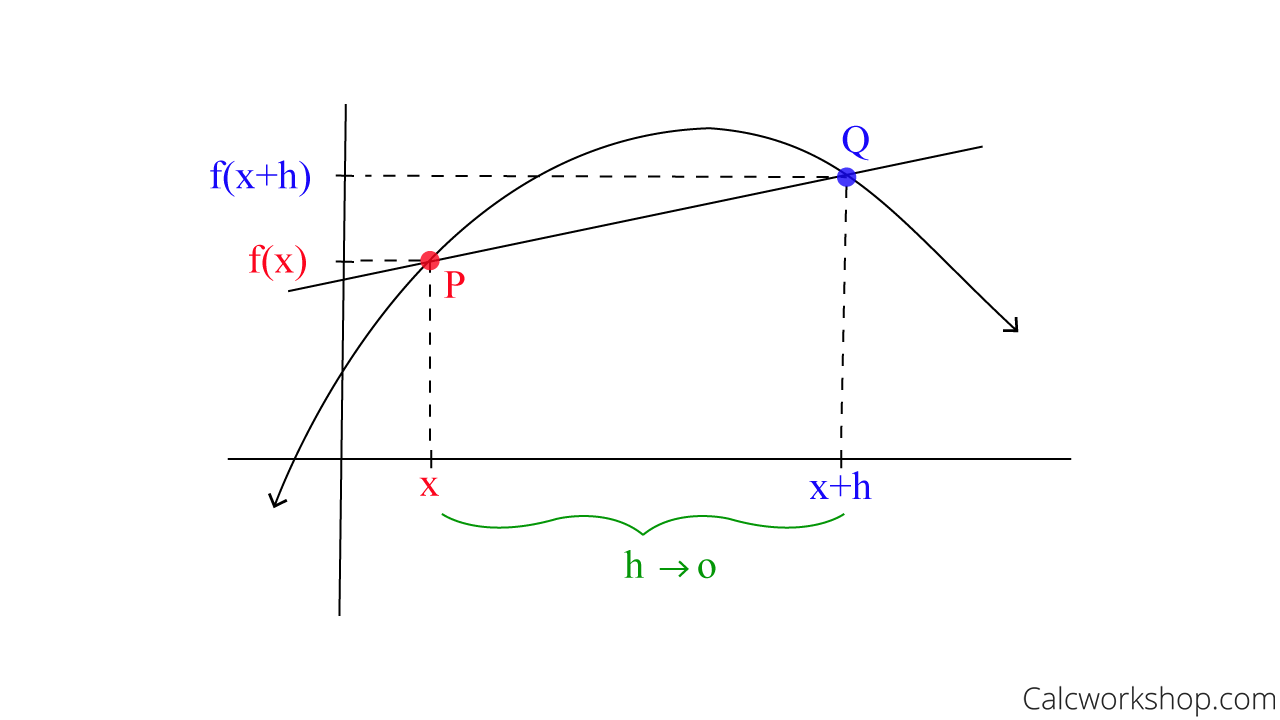
Let's formalize this. Suppose our point $P$ has coordinates $(a,f(a))$. We can choose a second point $Q$ nearby, with an x-coordinate of $a+h$, where $h$ is some small, non-zero number. The coordinates of $Q$ are $(a+h,f(a+h))$.

The slope of the secant line $PQ$, which we can call $m_{PQ}$, is given by the standard slope formula "rise over run":

This expression, $\frac{f(a+h)-f(a)}{h}$, is fundamental. It is called the difference quotient, and it represents the average rate of change of the function $f$ over the interval from $a$ to $a+h$.

To get the exact slope of the tangent line at $P$, we need to move the point $Q$ infinitely close to $P$. We do this by taking the limit as $h$ approaches 0.

3. The Definition of the Derivative

This limit, if it exists, gives us the slope of the tangent line and the instantaneous rate of change. We give it a special name: the derivative.

The following reading from a resource based on the Stewart textbook formally defines the tangent line and the derivative.

As you just read, we have two equivalent definitions for the derivative of a function $f$ at a number $a$, denoted $f^{\prime }(a)$ (read as "f prime of a"):

Definition of the Derivative at a Point

1. $f^{\prime }(a)={\lim }_{h\to 0}\frac{f(a+h)-f(a)}{h}$
2. $f^{\prime }(a)={\lim }_{x\to a}\frac{f(x)-f(a)}{x-a}$

Both formulas calculate the same value. The first form, using $h$, is generally more convenient for calculations. The value $f^{\prime }(a)$ has two crucial interpretations:

• Geometrically: $f^{\prime }(a)$ is the slope of the tangent line to the graph of $y=f(x)$ at the point $(a,f(a))$.
• Physically: $f^{\prime }(a)$ is the instantaneous rate of change of $f(x)$ with respect to $x$ when $x=a$.

4. Calculating the Derivative

Now, let's put the definition into practice. Calculating a derivative using the definition means setting up the difference quotient and evaluating the resulting limit. This process typically involves some algebraic simplification to handle the indeterminate form $\frac{0}{0}$ that arises when you first try to substitute $h=0$.

The video below demonstrates how to compute the derivative for a polynomial and a rational function using the $h\to 0$ definition.

Let's walk through the process for a new example: find the derivative of $f(x)=x^2-2x$ at $a=3$.

1. Write the definition:

   $$f^{\prime }(3)=\underset{h\to 0}{\lim }\frac{f(3+h)-f(3)}{h}$$

2. Substitute the function values:

   • $f(3)=3^2-2(3)=9-6=3$
   • $f(3+h)=(3+h{)}^2-2(3+h)$
     So, the limit becomes:
   $$f^{\prime }(3)=\underset{h\to 0}{\lim }\frac{[(3+h{)}^2-2(3+h)]-3}{h}$$

3. Simplify the numerator: First, expand the terms.

   $$(3+h{)}^2=9+6h+h^2$$ $$-2(3+h)=-6-2h$$

   Now, substitute these back into the numerator:

   $$\text{Numerator}=(9+6h+h^2)+(-6-2h)-3=(9-6-3)+(6h-2h)+h^2=4h+h^2$$

4. Cancel $h$: Our limit is now much simpler.

   $$f^{\prime }(3)=\underset{h\to 0}{\lim }\frac{4h+h^2}{h}=\underset{h\to 0}{\lim }\frac{h(4+h)}{h}=\underset{h\to 0}{\lim }(4+h)$$

5. Evaluate the limit: Now that we've cancelled the problematic $h$ in the denominator, we can substitute $h=0$.

   $$f^{\prime }(3)=4+0=4$$

So, the derivative of $f(x)=x^2-2x$ at $a=3$ is 4. This means the slope of the tangent line to the parabola at the point $(3,3)$ is exactly 4.

Conclusion

In this lesson, we have formally defined the derivative, one of the most important concepts in all of calculus. You have connected the intuitive ideas of tangent lines and instantaneous velocity to a precise mathematical definition built upon the concept of the limit.

Key Takeaways:

• The derivative of $f$ at $a$, written $f^{\prime }(a)$, solves both the tangent line problem and the instantaneous rate of change problem.
• The derivative is defined as the limit of the difference quotient:
  $f^{\prime }(a)={\lim }_{h\to 0}\frac{f(a+h)-f(a)}{h}$
• Geometrically, $f^{\prime }(a)$ is the slope of the tangent line to the graph of $y=f(x)$ at $x=a$.
• Calculating the derivative from the definition requires setting up the limit and using algebraic techniques (like expanding, factoring, or using conjugates) to resolve the indeterminate $\frac{0}{0}$ form.

In the example from the video, you saw the derivative of $f(x)=x^2-8x+9$ calculated at a general point $a$, which resulted in the expression $2a-8$. This suggests something powerful: what if we treat the point $a$ not as a fixed number, but as a variable? This would give us a new function that provides the slope at any point on the original curve. In our next lesson, we will explore this idea by defining the derivative as a function.