Graphing Derivatives

Introduction

In our last lesson, we established that the derivative of a function $f (x)$ , which we denote as $f^{'} (x)$ , is itself a function. This new function, $f^{'} (x)$ , gives us the slope of the tangent line to the original function $f (x)$ at any given point $x$ . We also explored the concept of differentiability, understanding that a function must be continuous and smooth (no corners, cusps, or vertical tangents) for its derivative to exist at a point.

Today, we will build on this foundation to develop a powerful visual skill: sketching the graph of the derivative function, $f^{'} (x)$ , by analyzing the graph of the original function, $f (x)$ . This is a purely graphical exercise that deepens the intuitive connection between a function and its rate of change. By the end of this lesson, you will be able to translate the geometric features of a function's graph into the graph of its derivative.

The Core Relationship: From Slopes to y-Values

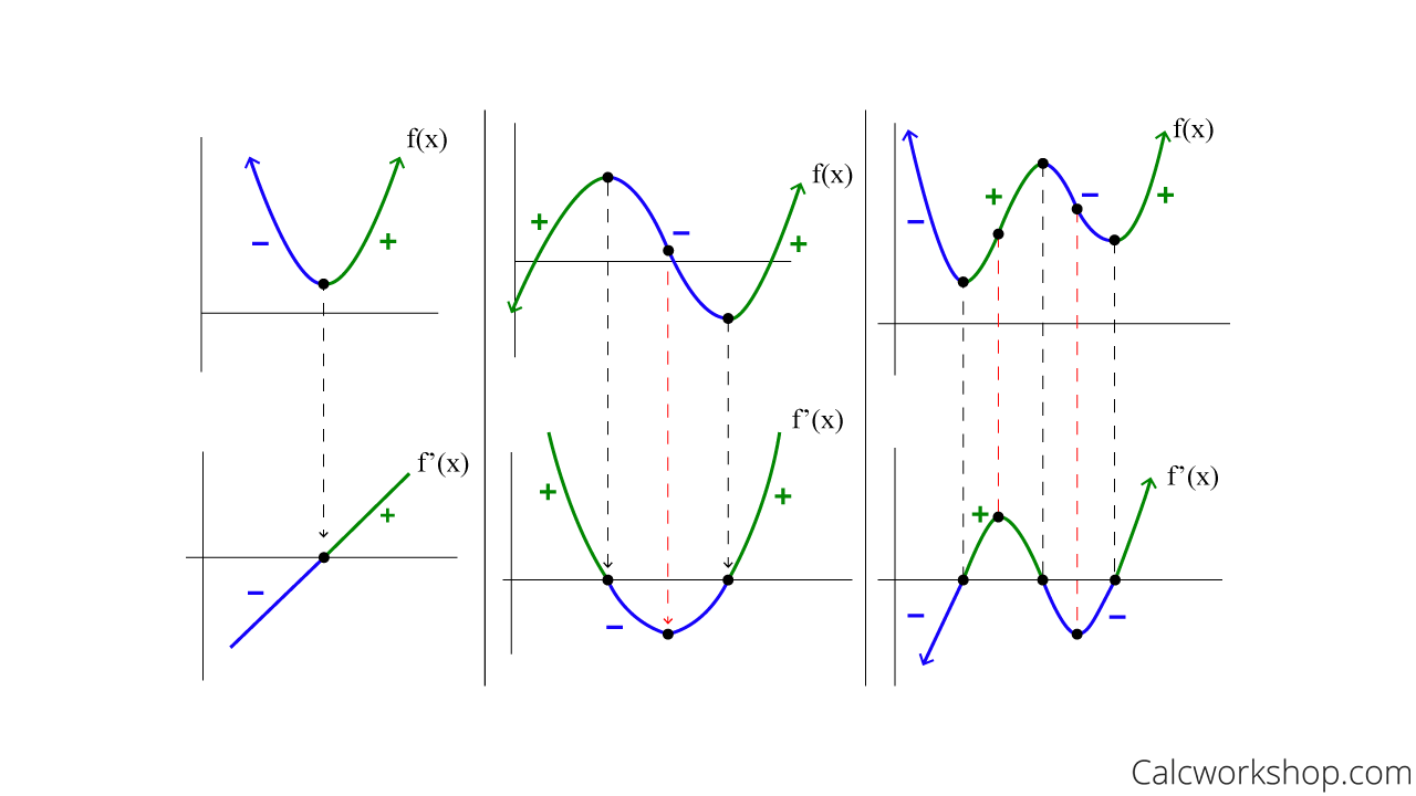
The most crucial concept for today's lesson is this: The y-value of the derivative graph $f^{'} (x)$ at a point is the value of the slope of the original function $f (x)$ at that same point.

Let's break this down into three key rules:

When $f (x)$ is increasing, the tangent lines to its graph have a positive slope. Therefore, the graph of $f^{'} (x)$ must be positive (i.e., above the x-axis).
When $f (x)$ is decreasing, the tangent lines have a negative slope. Therefore, the graph of $f^{'} (x)$ must be negative (i.e., below the x-axis).
When $f (x)$ has a horizontal tangent (e.g., at a local maximum or minimum), the slope is zero. Therefore, the graph of $f^{'} (x)$ must have a y-value of zero (i.e., it will touch or cross the x-axis).

This set of relationships is the fundamental dictionary we will use to translate between the two graphs.

These three pairs of graphs illustrate the core relationship. Notice how increasing sections on f(x) correspond to positive f'(x) values (above the x-axis), decreasing sections correspond to negative f'(x) values, and the flat tangent at the vertex of the parabola in the first example corresponds to an x-intercept for f'(x).

The following video provides a concise explanation of this principle.

Sketching Derivatives From Parent Functions - f f' f'' Graphs - f(x), Calculus

In this clip from The Organic Chemistry Tutor, pay close attention to the key sentence that summarizes our main idea.

Watch from the beginning until 01:51. The crucial takeaway is stated at the end: "The slope of f becomes the y-values of f'."

A Systematic Approach to Sketching

To sketch the derivative graph accurately, it helps to follow a structured process. We can think of it as a four-step algorithm.

Identify Horizontal Tangents: Locate all the points on the graph of $f (x)$ where the tangent line is horizontal (local maxima, minima, or saddle points). The x-coordinates of these points will be the x-intercepts (zeros) of the $f^{'} (x)$ graph. This is the best place to start, as it gives you concrete points for your sketch.
Analyze Increasing/Decreasing Intervals: Look at the intervals between and outside of the zeros you just found.
- In intervals where $f (x)$ is increasing, the graph of $f^{'} (x)$ will be above the x-axis.
- In intervals where $f (x)$ is decreasing, the graph of $f^{'} (x)$ will be below the x-axis.
Consider Steepness and Inflection Points: The steepness of $f (x)$ tells you the magnitude of $f^{'} (x)$ .
- If $f (x)$ is very steep, $f^{'} (x)$ will have a large absolute value (it will be far from the x-axis).
- If $f (x)$ has a gentle slope, $f^{'} (x)$ will be close to the x-axis.
- A point of inflection on $f (x)$ (where the curve changes from concave up to concave down, or vice-versa) corresponds to a point of maximum or minimum steepness. These points become the local extrema (peaks and valleys) on the graph of $f^{'} (x)$ .
Handle Non-Differentiable Points: As we learned in the previous lesson, if $f (x)$ has a sharp corner, a cusp, or a vertical tangent, then $f^{'} (x)$ is undefined at that x-value.
- A corner or cusp on $f (x)$ will create a jump discontinuity or a break in the graph of $f^{'} (x)$ .
- A vertical tangent on $f (x)$ will create a vertical asymptote on the graph of $f^{'} (x)$ .

The following image provides a good overview of these relationships on a more complex function.

This graph summarizes the key features. At points b and d, where the tangent is horizontal, f'(b) and f'(d) are zero. Where the function increases, f' > 0. Where it decreases, f' < 0. At point a, the cusp means f'(a) is undefined.

Walkthrough and Examples

Let's see this process in action. The best way to learn is by watching someone walk through the steps and then trying it yourself.

Sketching a Derivative from the Graph of a Function

In this video, Eddie Woo provides an excellent demonstration of sketching a derivative graph from a smooth curve. He uses a ruler to align the features, which is a great practical technique.

Watch from the start until 3:40. He will guide you through: Identifying the stationary points on f(x) to find the zeros of f'(x). Labeling the increasing (+) and decreasing (-) sections to determine where f'(x) is above or below the axis. Locating the point of inflection on f(x) to find the turning point of f'(x). Putting it all together to sketch the final graph.

Now, let's consider a function that isn't smooth everywhere. What happens at a sharp corner?

Sketching Derivatives From Parent Functions - f f' f'' Graphs - f(x), Calculus

This clip from The Organic Chemistry Tutor explains what happens when you have a function with non-differentiable points, like the absolute value function.

Watch the segment from 14:28 to 15:48. Note how the constant slope on the left side of the V-shape becomes a horizontal line at y=-1 on the derivative graph, and the constant slope on the right becomes a horizontal line at y=1. The sharp point at x=0 causes a jump discontinuity in the derivative graph.

For a final comprehensive overview, you can refer to this article. It includes a helpful summary table and worked examples for both smooth and piecewise functions.

Sketching Derivative Graphs: AP® Calculus AB–BC Review | Albert Blog & Resources

This resource from the Albert blog provides a structured strategy and a useful reference chart.

First, read the 4-Step Strategy. This formalizes the process we've been discussing. Then, review Worked Example #1 for a smooth curve and Worked Example #2 for a piecewise function. Finally, examine the Quick Reference Chart at the end. This table is an excellent summary to keep in mind.

Conclusion

Today we've transformed our algebraic understanding of the derivative into a powerful visual tool. You have learned to read the shape of a function's graph and translate it into a sketch of its derivative.

Key Takeaways:

The core principle is that the y-value of $f^{'} (x)$ represents the slope of $f (x)$ .
Zeros of $f^{'} (x)$ correspond to horizontal tangents on $f (x)$ (local extrema).
The sign of $f^{'} (x)$ (above/below x-axis) is determined by whether $f (x)$ is increasing or decreasing.
Extrema of $f^{'} (x)$ (peaks/valleys) correspond to inflection points on $f (x)$ (where steepness changes most).
Discontinuities in $f^{'} (x)$ (jumps, asymptotes) correspond to non-differentiable points on $f (x)$ (corners, cusps, vertical tangents).

So far, we have defined the derivative as a limit and learned to interpret it graphically. However, using the limit definition to calculate every derivative is cumbersome and inefficient. In our next lesson, we will begin developing a set of powerful shortcut rules, starting with the Power Rule, which will allow us to find derivative functions quickly and algebraically.

Recommended resources

Introduction

The Core Relationship: From Slopes to y-Values

A Systematic Approach to Sketching

Walkthrough and Examples

Conclusion