FP16/BFloat16 Mixed-Precision: Bandwidth and Throughput Impact

The Anatomy of a Floating-Point Number

To understand the trade-offs of different precision formats, we must first understand how a floating-point number is represented in binary. The IEEE 754 standard defines a number using three components:

1. Sign (S): A single bit indicating whether the number is positive (0) or negative (1).
2. Exponent: A set of bits that determines the magnitude or range of the number. It effectively positions the decimal (or binary) point.
3. Mantissa (or Fraction/Significand): A set of bits that determines the precision of the number—how many significant digits it can represent.

For the standard single-precision FP32 format, this is broken down into 1 sign bit, 8 exponent bits, and 23 mantissa bits.

The following video provides an excellent and detailed explanation of how these components work together, and then introduces the FP16 and BFloat16 formats.

FP16 vs. BFloat16: The Range vs. Precision Trade-off

As you saw in the video, moving from 32 bits to 16 bits requires a compromise. FP16 and BFloat16 represent two different approaches to this compromise.

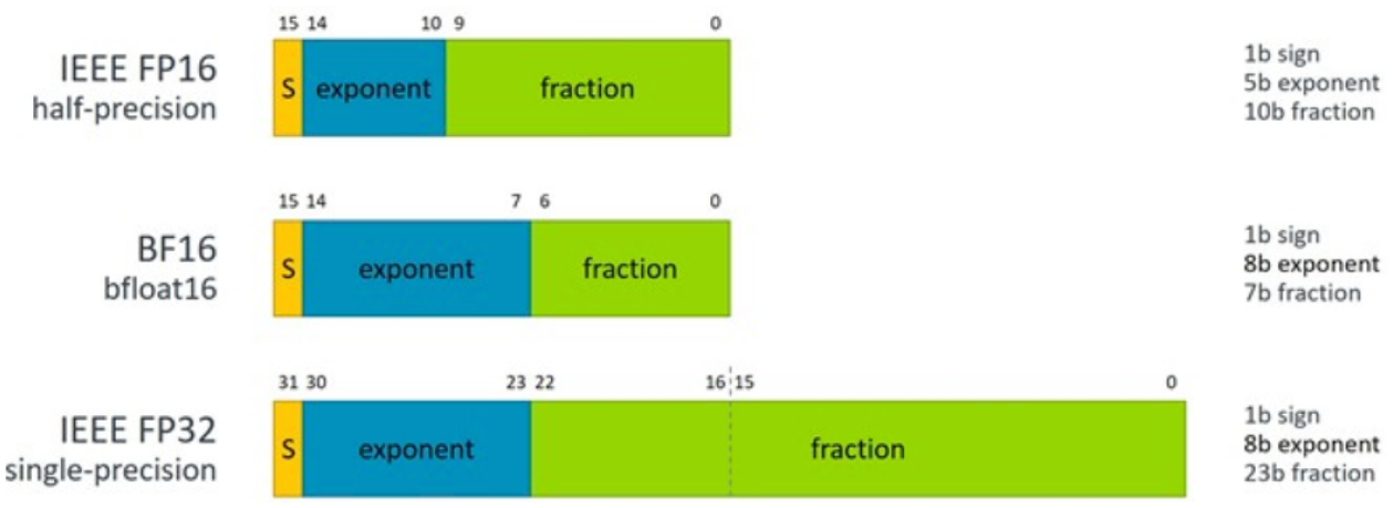
• FP16 (Half Precision): Allocates 5 bits for the exponent and 10 bits for the mantissa. Compared to FP32, it sacrifices both range and precision. Its drastically smaller exponent range ([-14, 15]) makes it susceptible to overflow (numbers too large) and underflow (numbers too small to be distinguished from zero).
• BFloat16 (Brain Float): Allocates 8 bits for the exponent and 7 bits for the mantissa. This is a clever trade-off: it maintains the exact same exponent range as FP32 while sacrificing even more precision than FP16.

For deep learning, gradients can have a very wide dynamic range. The ability of BFloat16 to represent both very large and very small numbers just like FP32 makes it inherently more stable and less prone to the underflow/overflow issues that plague FP16. This often simplifies training, as we will see later.

The Performance Payoff: Memory and Throughput

Using 16-bit floats offers two primary performance advantages, which you'll recognize from your understanding of GPU architecture.

1. Reduced Memory Footprint and Bandwidth: This is the most direct benefit. Halving the size of each number from 4 bytes (FP32) to 2 bytes (FP16/BF16) means:

   • You can fit larger models or use larger batch sizes within the same GPU memory.
   • You can transfer twice the number of elements between global memory and the SMs in the same amount of time, effectively doubling your memory bandwidth. This is crucial for memory-bound kernels.

2. Increased Compute Throughput via Tensor Cores: Modern NVIDIA GPUs include specialized hardware units called Tensor Cores. These are distinct from the general-purpose CUDA cores and are designed to accelerate one specific, critical operation: the matrix multiply-accumulate (MMA), $D=A\times B+C$.

   Tensor Cores achieve their incredible speed by operating on lower-precision inputs (like FP16 or BF16), often accumulating the result in a higher precision (like FP32) to maintain accuracy before optionally converting the final output back to a lower precision.

A single Tensor Core can perform many such operations in a single clock cycle, providing a massive increase in theoretical FLOPS (Floating-Point Operations Per Second) compared to what's possible with standard FP32 arithmetic on CUDA cores.

The Catch: Preserving Numerical Stability

If lower precision is so much faster, why not just switch everything to FP16 and call it a day? The answer lies in the numerical stability issues we hinted at earlier. Naively training a model entirely in FP16 often fails. Mixed-precision training is the set of techniques used to gain the speed of FP16 while maintaining the stability of FP32.

There are two primary problems to solve.

1. Weight Update Underflow

The update applied to a weight during training is typically learning_rate * gradient. This value can be extremely small. When you add this tiny update to a weight that is itself stored in FP16, the update can be too small to be represented by FP16's limited 10-bit mantissa. The result is that the addition does nothing, and the weight value effectively "stalls" and stops learning.

• The Solution: FP32 Master Weights
  The standard solution is to keep a master copy of the model weights in FP32. The forward and backward passes are performed with an FP16 copy of the weights to get the speed and memory benefits. However, when the optimizer is ready to update the weights, the FP16 gradients are converted to FP32 and applied to the FP32 master copy. This high-precision update is then copied back to the FP16 model for the next iteration.

Let's see a detailed explanation of this problem and its solution.

2. Gradient Underflow

The second, and often more severe, problem is that the activation gradients themselves can become so small during backpropagation that they fall below the minimum representable value of FP16. They are "flushed" to zero. This means the signal for learning is completely lost for those parts of the network.

• The Solution: Loss Scaling
  The solution here is to "shift" the entire distribution of gradients into the representable range of FP16. This is done by multiplying the loss value by a large scaling factor, S, before starting backpropagation. By the chain rule, this scales up all the gradients by S. Now, the small gradient values that would have underflowed are large enough to be represented in FP16.

  Of course, these scaled gradients cannot be used to update the weights directly. Before the optimizer step, the gradients are unscaled by dividing by S, ensuring the final weight update is numerically correct. This scaling can be done with a fixed factor, but modern frameworks use dynamic loss scaling, where the scaling factor S is automatically adjusted during training to find the optimal value that prevents underflow without causing overflow.

The Full Mixed-Precision Algorithm

Putting it all together, the full automatic mixed-precision (AMP) training algorithm implemented by modern frameworks like PyTorch and TensorFlow involves these steps:

1. Casting: Most operations in the forward and backward passes are run in FP16 or BFloat16 to leverage Tensor Cores and save memory. Certain numerically sensitive operations (e.g., reductions, softmax) are kept in FP32.
2. Loss Scaling: The loss is multiplied by a scaling factor S before the backward pass to prevent gradient underflow.
3. FP32 Master Weights: An FP32 copy of the model weights is maintained by the optimizer.
4. Gradient Unscaling: After the backward pass, the FP16 gradients are copied and unscaled back to their original magnitude in FP32.
5. Weight Update: The optimizer uses the unscaled FP32 gradients to update the FP32 master weights.
6. Copying back: The updated weights are copied back to the FP16 model for the next training iteration.

This combination of techniques allows deep learning models to achieve the performance benefits of 16-bit computation without sacrificing the accuracy and stability of 32-bit training.

Conclusion

In this lesson, we have moved from the world of pure FP32 computation into the pragmatic and performant domain of mixed-precision training. You now understand not only how 16-bit floating-point formats like FP16 and BFloat16 are structured, but also the critical trade-offs they make between numerical range and precision.

Key Takeaways:

• Floating-point numbers are defined by a sign, an exponent (range), and a mantissa (precision).
• FP16 sacrifices both range and precision, making it prone to underflow/overflow.
• BFloat16 maintains FP32's range at the cost of even lower precision, making it more robust for deep learning.
• Lower precision provides significant performance benefits through reduced memory bandwidth and, most importantly, by enabling computation on specialized Tensor Cores.
• Naive FP16 training fails due to weight update underflow and gradient underflow.
• Mixed-precision training solves these issues by using FP32 master weights and loss scaling, combining the speed of FP16 with the stability of FP32.

You've now seen the "what" and "why" of mixed precision at a conceptual level. In our next lesson, we will begin our deep dive into the "how" by learning to program the Tensor Cores directly, using low-level CUDA C++ intrinsics to write our own warp-level matrix multiplication kernels.