Numerically Stable Softmax with Two-Pass Parallel Reduction

Algorithm Strategy: A Two-Pass Parallel Reduction

For an input matrix of shape $M\times N$, a common and effective parallelization strategy is to launch one thread block for each of the $M$ rows. The threads within each block then work together to compute the softmax for their assigned row.

The numerically stable softmax formula is:

This naturally breaks down into a multi-step process for each row:

1. Find the maximum value: $\max (x)$.
2. Calculate the normalization factor (denominator): ${\sum }_j{e}^{x_j-\max (x)}$.
3. Compute the final output values: Divide each numerator $e^{x_i-\max (x)}$ by the normalization factor.

We will implement this using two distinct parallel reduction phases within a single CUDA kernel. This approach is a significant step up from a naive implementation where each thread would redundantly read the entire row multiple times.

Let's watch a brief segment that introduces this reduction-based approach.

Kernel Structure and Pass 1: Finding the Maximum

We will launch our kernel with M blocks and a chosen block_size (e.g., 256 or 512). Inside the kernel, the first step for each block is to find the maximum value of its assigned row.

The process is as follows:

1. Local Reduction: Each thread in the block processes a subset of the row elements. It iterates through its assigned elements and finds a local maximum (local_max).
2. Block-wide Reduction: The threads then collaborate to "reduce" their local_max values into a single global_max for the entire row. This is done using shared memory.

Let's review how a block-wide reduction using shared memory works. The following resource provides an excellent, detailed walkthrough.

With this reduction pattern in mind, the first half of our kernel looks like this in pseudocode:

__global__ void softmax_kernel(float* input, float* output, int M, int N) {
    // Each block processes one row
    int row = blockIdx.x;
    int tid = threadIdx.x;

    // Allocate shared memory for the reduction
    __shared__ float smem[BLOCK_SIZE];

    // --- PASS 1: Find Maximum Value ---

    // 1. Local Reduction
    float local_max = -INFINITY;
    for (int i = tid; i < N; i += blockDim.x) {
        local_max = max(local_max, input[row * N + i]);
    }

    // 2. Block-wide Reduction
    smem[tid] = local_max;
    __syncthreads(); // Ensure all local_max values are in shared memory

    // The reduction loop from the article goes here...
    for (int stride = blockDim.x / 2; stride > 0; stride /= 2) {
        if (tid < stride) {
            smem[tid] = max(smem[tid], smem[tid + stride]);
        }
        __syncthreads();
    }

    // The global max for the row is now in smem[0]
    float global_max = smem[0];
    __syncthreads(); // Ensure all threads see the final max
    
    // ... Pass 2 and Final Computation will follow
}

Pass 2: Calculating the Normalization Factor

After Pass 1, global_max (the row's maximum value) is available to all threads in the block. Now we can proceed to the second reduction pass to compute the denominator, which we'll call norm.

The logic is identical to Pass 1, but with two key differences:

• The operation is summation (+) instead of max.
• The value each thread accumulates locally is $e^{x_i-\text{global\_max}}$.

The pseudocode for this second pass continues from where we left off:

// (Continued from Pass 1)
// float global_max = smem[0];
// __syncthreads();

// --- PASS 2: Find Normalization Factor ---

// 1. Local Reduction
float local_norm = 0.0f;
for (int i = tid; i < N; i += blockDim.x) {
    local_norm += expf(input[row * N + i] - global_max);
}

// 2. Block-wide Reduction for the sum
smem[tid] = local_norm;
__syncthreads(); // Ensure all local_norm values are in shared memory

// Reduction loop for summation...
for (int stride = blockDim.x / 2; stride > 0; stride /= 2) {
    if (tid < stride) {
        smem[tid] += smem[tid + stride];
    }
    __syncthreads();
}

// The global norm for the row is now in smem[0]
float global_norm = smem[0];
__syncthreads(); // Ensure all threads see the final norm

Final Computation and Write-Out

With both global_max and global_norm computed and available to all threads, the final step is straightforward. We perform a third and final traversal of the row, where each thread calculates the final softmax value for its assigned elements and writes them to global memory.

// (Continued from Pass 2)
// float global_norm = smem[0];
// __syncthreads();

// --- Final Computation and Write ---
for (int i = tid; i < N; i += blockDim.x) {
    int index = row * N + i;
    output[index] = expf(input[index] - global_max) / global_norm;
}

This completes the kernel. While it involves three loops over the data, it's considered a "two-pass reduction algorithm" because its core parallel logic consists of two block-wide reduction operations. This implementation is vastly more efficient than a naive one, as it minimizes redundant reads from global memory and effectively parallelizes the two most expensive parts of the computation.

Optimizations and Further Thoughts

The implementation we've designed is a solid, understandable, and correct parallel algorithm. However, in the world of high-performance computing, the optimization journey is never truly over.

Online Softmax:
One major optimization is to fuse the two reduction passes into one. This is known as the "online softmax" method. In a single pass over the data, it's possible to maintain a running estimate of both the maximum and the normalization factor, applying a correction to the norm whenever a new maximum is found.

Warp-Level Primitives:
Another powerful optimization is to use warp-level shuffle instructions (__shfl_down_sync) for the reduction. As you learned in Module 6, these allow threads within a warp to exchange data directly through registers, avoiding the overhead of writing to and reading from shared memory. A highly optimized kernel would first perform a reduction within each warp using shuffles, and then use shared memory only to reduce the results from each warp.

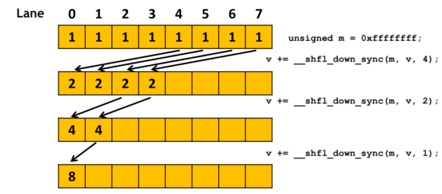
You can explore a kernel that uses these shuffle instructions in the resource Learning CUDA by optimizing softmax: A worklog under "Kernel 4 - Shuffle instructions".

Conclusion

In this lesson, you have translated the theoretical concept of a numerically stable softmax into a concrete, parallel CUDA kernel. You designed a block-per-row strategy and correctly applied the parallel reduction primitive twice: once to find the maximum value, and a second time to find the normalization factor.

Key Takeaways:

• A numerically stable softmax can be implemented in CUDA using a two-pass parallel reduction algorithm.
• The strategy of assigning one block per row allows for efficient intra-block collaboration.
• Pass 1 performs a max reduction using shared memory to find the row's maximum value.
• Pass 2 performs a sum reduction using shared memory to calculate the normalization factor based on the result of Pass 1.
• A final pass computes the output values and writes them to global memory.
• This approach is a robust and performant baseline, which can be further optimized with advanced techniques like online softmax and warp-level primitives.

With your understanding of kernel fusion, normalization, and now softmax, you are building a solid toolkit for implementing the core components of modern AI models. In our next lesson, we will explore another critical concept for performance: the use of lower-precision data types like FP16 and BFloat16 in mixed-precision computing.