Building a KNN Baseline with Scikit-learn

The Intuition Behind K-Nearest Neighbors

At its core, the KNN algorithm operates on a simple, relatable principle: a data point is likely to be similar to the data points closest to it. You could summarize it as, "Tell me who your neighbors are, and I'll tell you who you are."

When we want to classify a new, unseen data point, KNN performs the following steps:

1. It calculates the distance from the new point to every single point in the training dataset.
2. It identifies the 'k' points from the training data that are closest to the new point (its "nearest neighbors").
3. It holds a "vote" among these 'k' neighbors. The new data point is assigned the class label that is most common among its neighbors (the majority class).

The following video from the codebasics channel provides an excellent visual explanation of this process using the famous Iris dataset.

As you saw, the algorithm's behavior is governed by two key choices: the value of 'k' and the method used to measure distance.

The Key Hyperparameters: 'k' and Distance Metric

1. Choosing 'k'

The number of neighbors, 'k', is a hyperparameter that you, the modeler, must choose. This choice has a significant impact on the model's behavior and is a classic example of the bias-variance tradeoff we've discussed previously.

• A small 'k' (e.g., k=1) makes the model highly flexible and sensitive to local variations in the data. The decision boundary can become very complex and "noisy." This can lead to high variance and overfitting, as the model might be fitting to noise and outliers rather than the underlying pattern.
• A large 'k' (e.g., k=20) makes the model consider a much larger neighborhood for its vote. This smooths out the decision boundary, making the model more robust to noise but less sensitive to local patterns. This can lead to high bias and underfitting, as the model might become too general and fail to capture important distinctions in the data.

Finding the optimal 'k' is a task for model evaluation and hyperparameter tuning, which we will cover in detail in a future module. For now, it's crucial to recognize this tradeoff.

2. Measuring Distance

The notion of "closeness" is formalized by a distance metric. While several metrics exist, the most common is the Euclidean distance—the straight-line distance between two points in a multi-dimensional space. Given your background in mathematics, you'll recognize this as a generalization of the Pythagorean theorem. For two points, $p$ and $q$, in an n-dimensional feature space, the Euclidean distance is:

This formula underscores a critical prerequisite for KNN: feature scaling. If one feature (e.g., salary in dollars) is on a much larger scale than another (e.g., years of experience), it will dominate the distance calculation, effectively making the other features irrelevant. Therefore, it's standard practice to scale your features (e.g., using standardization or normalization) before applying KNN.

Implementing KNN with Scikit-learn

Now, let's move from theory to practice. We'll use scikit-learn to build a KNN classifier for a synthetic dataset. The GeeksforGeeks article, "k-nearest neighbor algorithm using Sklearn," provides a clean, step-by-step guide that we will follow.

Let's synthesize those steps into a single, corrected, and complete code block. This is the workflow you will use for many of your projects.

# 1. Import necessary libraries
import numpy as np
import matplotlib.pyplot as plt
import seaborn as sns
import pandas as pd
from sklearn.datasets import make_moons
from sklearn.model_selection import train_test_split
from sklearn.preprocessing import StandardScaler
from sklearn.neighbors import KNeighborsClassifier
from sklearn.metrics import accuracy_score




# 2. Generate and visualize data
X, y = make_moons(n_samples=300, noise=0.3, random_state=42)




# 3. Feature Scaling (Crucial for KNN)
# We scale the entire dataset before splitting
scaler = StandardScaler()
X_scaled = scaler.fit_transform(X)




# 4. Split data into training and testing sets
X_train, X_test, y_train, y_test = train_test_split(
    X_scaled, y, test_size=0.3, random_state=42, stratify=y
)




# 5. Instantiate and train the KNN model
# The "fit" process for KNN is just storing the training data
knn = KNeighborsClassifier(n_neighbors=5)
knn.fit(X_train, y_train)




# 6. Make predictions on the test set
y_pred = knn.predict(X_test)




# 7. Evaluate the model
accuracy = accuracy_score(y_test, y_pred)
print(f"Test Accuracy (k=5): {accuracy:.2f}")




# You can also use the model's score method
print(f"Model score on test data: {knn.score(X_test, y_test):.2f}")

This code encapsulates the entire process: creating data, preprocessing it (scaling), splitting it for validation, training a model, and evaluating its performance. This fit/predict/score pattern is the heart of the scikit-learn API and you will see it again and again.

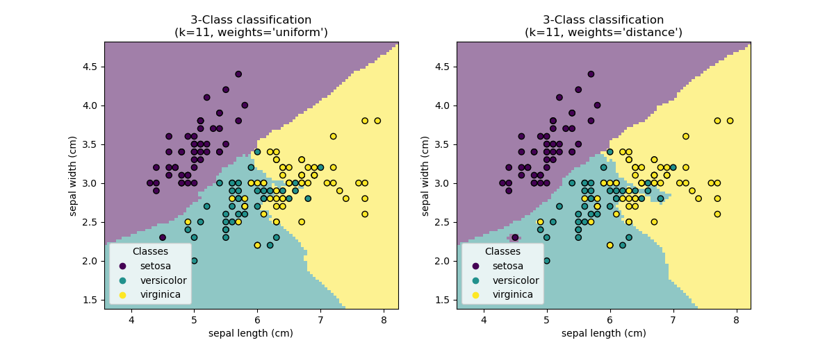
Advanced Tweak: Weighting Neighbors

In the basic KNN algorithm, each of the 'k' neighbors gets an equal vote. But what if one neighbor is much closer than the others? It seems intuitive that closer neighbors should have more influence.

Scikit-learn allows for this through the weights hyperparameter.

• weights='uniform' (the default): All neighbors have an equal vote.
• weights='distance': Each neighbor's vote is weighted by the inverse of its distance. Closer neighbors get a stronger vote.

This simple change can often lead to a more nuanced and accurate decision boundary.

Conclusion

In this lesson, you've successfully transitioned from setting up your environment to building and evaluating your first machine learning model. You have not only implemented a KNN classifier but also delved into the reasoning behind its core components.

Here are the main takeaways:

• KNN is an intuitive, instance-based learning algorithm that classifies new data based on a majority vote of its 'k' nearest neighbors.
• The choice of 'k' is a critical hyperparameter that controls the bias-variance tradeoff.
• Feature scaling is essential for distance-based algorithms like KNN to prevent features with large scales from dominating the distance calculation.
• The scikit-learn API provides a simple and consistent fit, predict, score interface for building and evaluating models.
• A baseline model like KNN is a crucial first step in any machine learning project, providing a benchmark against which more complex models can be measured.

You have now completed the first module of this course, laying a solid foundation in the core concepts and practices of machine learning.

In our next lesson, we will begin the "Data Preprocessing and Exploratory Analysis" module. We'll move from synthetic data to real-world datasets, learning how to load and inspect a tabular dataset using pandas, which is the foundational skill for any data-driven modeling.