Indexing for Faster Data Retrieval

The Problem: Why Is Searching a Large Table Slow?

Imagine you have a massive table, say, employees, with millions of records. When you run a query like SELECT * FROM employees WHERE employee_id = 50021;, how does the database find that one specific row?

If there's no index on the employee_id column, the database has no choice but to perform a full table scan. It's like looking for a single word in a book by reading it from the first page to the last. The database has to load every single record from the disk and check if its employee_id is 50021.

This process is slow primarily because of disk I/O (Input/Output). Reading data from a spinning hard drive or even an SSD is orders of magnitude slower than reading data from memory (RAM). The database reads data from disk in fixed-size chunks called pages or blocks. A full table scan on a large table might require reading thousands or millions of these pages, which is a major performance bottleneck.

To build a solid foundation for understanding this problem, let's explore it with some concrete numbers.

As the article demonstrates, even a simple index—a separate, smaller table containing just the indexed column value and a pointer to the full row—can provide a significant performance boost by reducing the amount of data that needs to be read from disk.

From a Simple List to an Efficient Tree

The single-level index works well, but what happens when the table grows so large that even the index itself becomes too big to scan quickly? We're back to the same problem, just on a smaller scale.

The solution is to create an index on the index! This concept of a multi-level index is the key to understanding modern database indexes. By creating a hierarchy, we can quickly navigate to the right section of the index without scanning the whole thing. This hierarchical structure is, in essence, a tree.

Let's watch a short video that illustrates this evolution of thought, from a simple (and slow) data structure to a more sophisticated one.

The B-Tree: A Data Structure Designed for Disk

The video introduced the star of our lesson: the B-Tree. Most relational databases use a variant of the B-Tree for their standard indexes. Its design is a brilliant piece of engineering tailored specifically for the limitations of disk-based storage.

Here are the key characteristics that make B-Trees so effective:

1. They are "fat" and "shallow." Unlike a binary tree where each node has at most two children, a B-Tree node can have hundreds or even thousands of children. This means the tree is very wide, but also very short (low height). A B-Tree for a table with hundreds of millions of rows might only be 3 or 4 levels deep.
2. Nodes map to disk pages. The size of a B-Tree node is typically designed to match the size of a disk page (e.g., 16KB). When the database needs to look at a node, it loads a single page from disk.
3. They are self-balancing. The B-Tree has rules for insertion and deletion that ensure the tree remains balanced. This guarantees that the path from the root to any leaf is always roughly the same length, providing predictable O(log n) search performance.

So, how does this speed up a search?

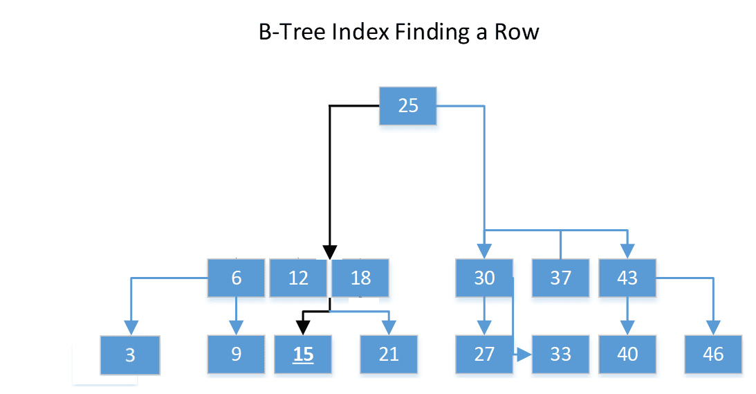
When you search for a value using a B-Tree index, the database performs an index seek:

1. It starts at the root node (which is usually kept in memory).
2. It follows pointers down the tree, loading just one node (page) per level.
3. In just a few disk reads (equal to the height of the tree), it can pinpoint the exact location of the data on disk.

Instead of reading all 10,000 pages for a full table scan, the database might only need to read 3 or 4 pages to find your row. This is the source of the massive performance gain.

A Practical Improvement: The B+ Tree

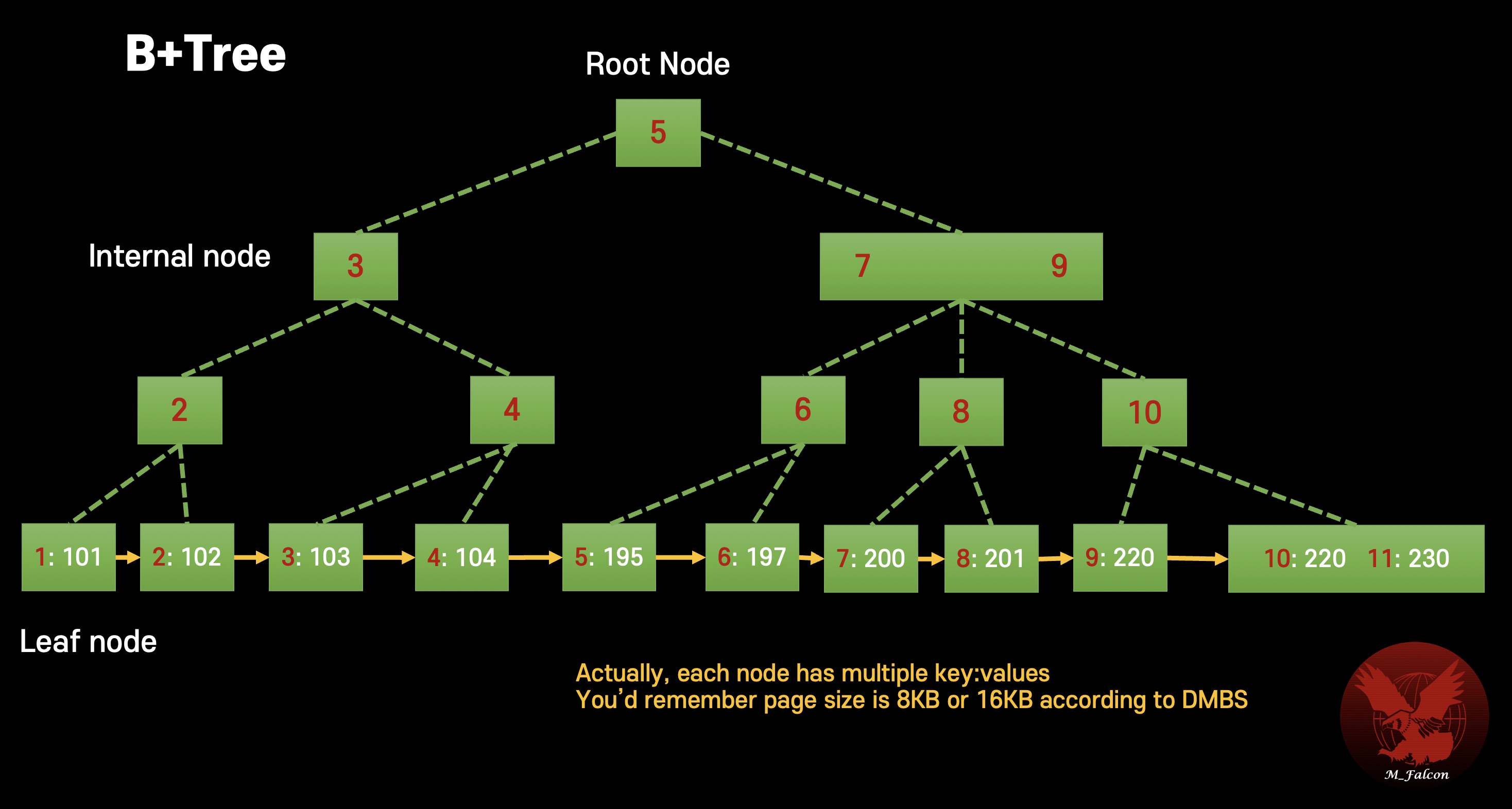
While we've been discussing B-Trees, it's important to know that most modern databases like MySQL and PostgreSQL actually use a variation called a B+ Tree. It has two key differences that make it even more suitable for database workloads:

1. Data is stored only in the leaf nodes. The internal (non-leaf) nodes only store keys for routing, making them smaller. This allows more keys to fit in each internal node, which can make the tree even wider and shallower.
2. Leaf nodes are linked together. The leaf nodes form a doubly-linked list. This is extremely efficient for range queries (e.g., WHERE age BETWEEN 30 AND 40), as the database can find the first value (30) and then just follow the linked list to get the rest, without having to traverse back up the tree.

Let's return to our first resource to see a clear explanation of these concepts.

Conclusion

In this lesson, we peeled back the layers of database indexing to understand the "low-level why" of its performance benefits. You now have a mental model that connects the abstract idea of an "index" to the concrete engineering of disk I/O, page management, and tree-based data structures.

Key Takeaways:

• Searching a table without an index requires a full table scan, which is slow due to the high number of disk I/O operations needed to read every page of the table.
• An index is a separate data structure that provides a fast lookup path from a key value to the location of the corresponding data row.
• B-Trees (and more commonly, B+ Trees) are the go-to data structure for indexes because they are self-balancing and optimized for disk. Their wide and shallow structure minimizes the number of disk reads required to find a value, reducing search complexity from linear O(n) to logarithmic O(log n).
• The key to an index's speed is its ability to drastically reduce disk I/O by replacing a massive scan with a few targeted reads.

Preview of the Next Lesson:
Now that you understand how indexes work under the hood, the next logical step is to learn how to create and manage them. In our next lesson, "Create a single-column or composite index to optimize a query," we will move from theory to practice. You'll learn the SQL syntax for creating indexes and begin to develop the intuition for which columns in a table are good candidates for indexing.