Hello and welcome to your first lesson. This course is designed to give you a deep, rigorous understanding of the principles that govern organic chemistry, starting from the quantum mechanical foundations of atomic structure. Given your interest in the "why" behind chemistry and your background in mathematics, we will begin by exploring exactly where the familiar shapes of atomic orbitals come from.
Today, we will answer the question: How do the solutions to the Schrödinger equation lead to the spherical 's' orbitals, the dumbbell-shaped 'p' orbitals, and the more complex 'd' orbitals? By the end of this lesson, you will be able to explain these shapes not as arbitrary rules, but as direct consequences of the mathematical framework of quantum mechanics.
1. The Schrödinger Equation in Three Dimensions
At the heart of quantum chemistry is the time-independent Schrödinger equation, which describes the wavefunction () and energy () of a quantum system. For a single electron in an atom (like hydrogen), this equation is:
Here, is the reduced Planck constant, is the electron's mass, is the Laplacian operator (representing kinetic energy), and is the potential energy. For an electron orbiting a nucleus, the potential is the Coulomb potential, , which depends only on the distance from the nucleus.
This spherical symmetry of the potential makes it far more practical to solve the equation in spherical coordinates rather than Cartesian coordinates .
2. The Strategy: Separation of Variables
The key to solving this complex partial differential equation is a powerful mathematical technique called separation of variables. Because the potential energy only depends on the radial coordinate , we can hypothesize a solution where the wavefunction is a product of a purely radial function, , and a purely angular function, .
Substituting this into the Schrödinger equation and rearranging allows us to separate the equation into two independent ordinary differential equations:
- The Radial Equation: Involves only and determines the energy and size of the orbital.
- The Angular Equation: Involves only and and determines the shape of the orbital.
To see the formal mathematical derivation of this separation, please start by reading the following text.
Chapter 10 The Hydrogen Atom The Schrodinger Equation ...
This document, 'Chapter 10 The Hydrogen Atom', lays out the mathematical framework for solving the Schrödinger equation. It will show you how the equation is set up in spherical coordinates and how the separation of variables technique is applied.
Please read the first two pages, starting from the beginning of 'Chapter 10 The Hydrogen Atom' up to the end of equation (10-7). Focus on understanding how the full Schrödinger equation (10-2) is broken down into the radial equation (10-6) and the angular equation (10-7). Don't worry about the linear algebra arguments for now; focus on the variable separation process.
For a dynamic and narrated walkthrough of this crucial separation technique, the following video provides an excellent conceptual explanation.
The Hydrogen Atom, Part 2 of 3: Solving the Schrodinger Equation
The video 'The Hydrogen Atom, Part 2 of 3: Solving the Schrodinger Equation' by Richard Behiel provides a clear visualization and explanation of the separation of variables.
Watch the segment from 27:36 to 30:41. The presenter walks through the logic of separating the Schrödinger equation into a radial part and an angular part, emphasizing why this is possible and what it means.
3. The Angular Equation: Spherical Harmonics and Orbital Shapes
Since our goal is to understand orbital shapes, we will now focus on the angular equation. Its solutions are a famous set of functions in mathematical physics known as the spherical harmonics, . These functions dictate the angular probability distribution of the electron.
The angular equation itself can be separated again, this time into equations for and . This process reveals the origin of two of the four quantum numbers.
To see how this works and how it leads directly to the functions that define orbital shapes, please watch the following video.
Spherical harmonics for Schrodinger equation
This video, 'Spherical harmonics for Schrodinger equation' by Professor Nano, provides a concise and clear derivation of the spherical harmonics and visualizes them as the familiar s, p, and d orbitals.
Watch the entire video (approximately 11 minutes). It's the core of this lesson. Pay close attention to: How the angular equation is separated into heta and \phi parts (3:24). How the boundary condition on \phi quantizes the magnetic quantum number, m_l (5:50). How the solutions to the heta equation (Associated Legendre polynomials) lead to the quantization of the angular momentum quantum number, l (6:40). Crucially, how linear combinations of the complex solutions produce the real p- and d-orbitals we use in chemistry (9:18).
Let's summarize and solidify the key insights from the video:
Quantum Numbers from the Angular Solution
-
The Magnetic Quantum Number, : The equation for has solutions of the form . For the wavefunction to be physically realistic, it must be single-valued, meaning it must have the same value at and . This condition is only met if is an integer (). This is a beautiful example of a physical constraint leading directly to quantization.
-
The Angular Momentum Quantum Number, : The equation for (the Associated Legendre equation) only has physically well-behaved solutions (ones that don't become infinite) if is a non-negative integer () and if . This quantum number, , determines the overall shape of the orbital.
Visualizing the Solutions as Orbitals
The squared modulus of the spherical harmonics, , gives the angular probability density.
-
s-orbitals ():
When , the only possible value for is 0. The function is a constant, independent of and .
This means the probability is the same in every direction, resulting in a spherical shape. -
p-orbitals ():
When , can be -1, 0, or +1.- The case corresponds to the orbital, which has its lobes of maximum probability along the z-axis.
- The and solutions are complex-valued. Chemists take linear combinations of them to form two real-valued, orthogonal orbitals:
These combinations result in the familiar dumbbell shapes oriented along the x and y axes.
-
d-orbitals ():
When , can be -2, -1, 0, +1, +2, giving five d-orbitals.- The case gives the orbital.
- Linear combinations of the cases give the and orbitals.
- Linear combinations of the cases give the and orbitals.
The following resources provide excellent static visualizations of these shapes.
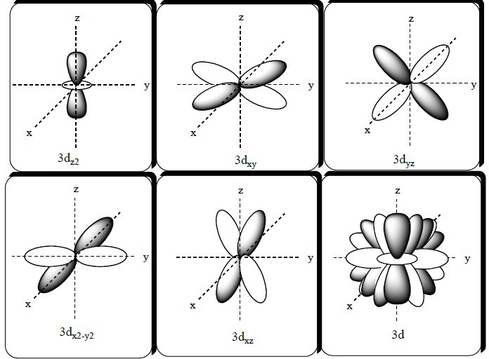
2.2.2: Quantum Numbers and Atomic Wave Functions
This webpage from LibreTexts, 'Quantum Numbers and Atomic Wave Functions', provides clear tables and diagrams that summarize the orbital shapes and connect them to their quantum numbers.
Scroll down to the heading 'Angular contribution, Y_{l, m_l}( heta, \phi)...' and review the table and images. This will reinforce the connection between the quantum numbers (l, m_l), the mathematical functions, and the final orbital shapes you saw in the video.
4. The Radial Component: Size and Nodes
While the angular function gives the orbital its shape, the radial function determines its size and how the probability changes with distance from the nucleus.
Solving the radial equation introduces the principal quantum number, (), which is the primary determinant of the electron's energy and the orbital's size. The solutions, , involve functions called Associated Laguerre polynomials.
A key feature of the radial functions are radial nodes: spherical surfaces where the probability of finding the electron is zero (). The number of radial nodes for an orbital is given by the formula:
For example, a 1s orbital () has 0 radial nodes. A 2s orbital () has 1 radial node, which you can visualize as a spherical shell separating an inner region of electron density from an outer one.
Test your understanding!
How many radial nodes does a 3p orbital have? How many angular nodes?
Show answer
For a 3p orbital, and .
- Number of radial nodes = .
- Number of angular nodes = .
The total number of nodes is .
Conclusion
In this lesson, we have taken a deep dive into the quantum mechanical origins of atomic orbitals. You now have the foundational knowledge to see orbitals not just as convenient pictures, but as graphical representations of the mathematical solutions to the Schrödinger equation.
Key Takeaways:
- The shapes of atomic orbitals are determined by the angular part of the wavefunction, , which are solutions to the angular Schrödinger equation.
- These solutions, the spherical harmonics, are indexed by the quantum numbers and .
- The angular momentum quantum number determines the fundamental shape (s, p, d, f) and the number of angular nodes.
- The magnetic quantum number determines the orientation of the orbital in space (e.g., ).
- The size and radial structure (radial nodes) of an orbital are determined by the radial part of the wavefunction, , which depends on the quantum numbers and .
By understanding this mathematical origin, you are well-equipped to appreciate the more nuanced aspects of chemical bonding that we will explore throughout this course.
Preview of the Next Lesson:
Now that we have a description for the orbitals (the "houses" for electrons), our next step is to understand the rules that govern how electrons occupy these orbitals. In the next lesson, we will introduce the concept of electron spin and explore the fundamental principles—the Pauli exclusion principle and Hund's rule—that dictate electron configurations in atoms.