BFS for Shortest Path in Unweighted Graphs

The Shortest Path Problem

In an unweighted graph, the "length" or "cost" of any path is simply the number of edges it contains. The shortest path problem, therefore, is about finding a path between a source node and a destination node that consists of the minimum number of edges.

There are several variations of this problem, but today we will focus on the single-source shortest path problem, where we find the shortest path from a starting node to all other nodes. By solving this, we can easily find the specific path to any single destination.

Let's begin with a video that frames the problem and introduces the key idea.

Why BFS Guarantees the Shortest Path

The key insight is that BFS naturally discovers nodes in increasing order of their distance from the source. It explores all nodes at distance 1, then all nodes at distance 2, and so on. This creates an "expanding wavefront" moving out from the source node.

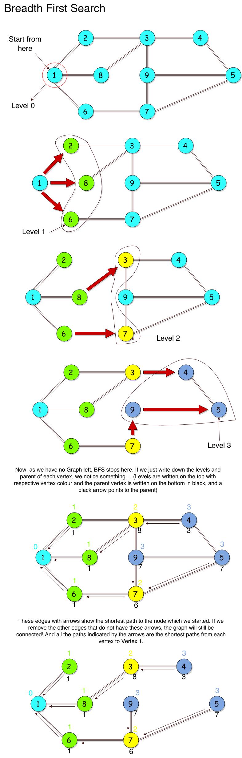
Because of this orderly, level-by-level exploration, the first time BFS encounters any node, it is guaranteed to have found a shortest path to it. If a shorter path existed, BFS would have had to traverse fewer edges, meaning it would have discovered the node at an earlier level, which is a contradiction.

For a great visual analogy that helps solidify this intuition, let's watch a brief clip.

The Algorithm: Modifying BFS for Path-Finding

A standard BFS traversal tells you if a path exists. To reconstruct the path itself, we need to make a small but crucial modification: we must keep track of how we arrived at each node.

We can achieve this by using a parent or predecessor data structure (like a dictionary or an array). When our BFS moves from a node u to its neighbor v, we record that we reached v from u by setting parent[v] = u.

The algorithm looks like this:

1. Initialization:

   • Create a queue and add the start node.
   • Create a visited set to avoid cycles and redundant work, adding the start node to it.
   • Create a parent dictionary to store the path. Initialize it with parent[start] = None.

2. Traversal:

   • While the queue is not empty:
     • Dequeue the current node, u.
     • If u is the goal node, stop the search. You've found the shortest path.
     • For each neighbor of u:
       • If the neighbor has not been visited:
         • Add it to the visited set.
         • Set parent[neighbor] = u.
         • Enqueue the neighbor.

3. Path Reconstruction:

   • If the goal node was found, trace your steps backward from goal using the parent dictionary until you reach the start node.
   • This backward trace gives you the path in reverse, so you'll need to reverse it to get the final path from start to goal.

The following video segments walk through these data structures and the path reconstruction process in detail.

A Complete Example and Implementation

Let's tie everything together. The article "Shortest path in an unweighted graph" from GeeksforGeeks provides a concise summary and code structure. We'll then look at a clean Python implementation.

Based on this logic, here is a complete Python implementation. This function takes a graph (represented as an adjacency list), a start node, and a goal node, and returns the shortest path as a list of nodes.

from collections import deque

def bfs_shortest_path(graph, start, goal):



    # Keep track of explored nodes
    explored = {start}
    



    # Queue for BFS, storing paths
    # The queue will store the path taken to reach a node
    queue = deque([[start]])
    
    if start == goal:
        return [start]
    
    while queue:



        # Get the first path from the queue
        path = queue.popleft()
        node = path[-1]
        



        # Go through all neighbors
        for neighbour in graph.get(node, []):
            if neighbour not in explored:



                # Create a new path by extending the current one
                new_path = list(path)
                new_path.append(neighbour)
                queue.append(new_path)
                



                # Mark neighbor as explored
                explored.add(neighbour)
                



                # If we've reached the goal, return the path
                if neighbour == goal:
                    return new_path
                    



    # If the queue becomes empty and goal was not found
    return "No path found between the nodes."




# Example Usage:
graph = {
    'A': ['B', 'C'],
    'B': ['A', 'D', 'E'],
    'C': ['A', 'F'],
    'D': ['B'],
    'E': ['B', 'F'],
    'F': ['C', 'E', 'G'],
    'G': ['F']
}

print(f"Shortest path from A to G: {bfs_shortest_path(graph, 'A', 'G')}")



# Expected output: ['A', 'C', 'F', 'G'] or ['A', 'B', 'E', 'F', 'G']
# The algorithm finds one of the shortest paths. In this case, there are two of length 3.
# Depending on neighbor order, it might find ['A', 'C', 'F', 'G']

Note: This implementation stores the entire path in the queue, which is intuitive but can use more memory than the parent-pointer method. For your GNN work, understanding the concept is key, and both implementation strategies are valid ways to think about it.

Conclusion

Congratulations on completing the first module! You have built a solid foundation in graph theory, moving from basic definitions to implementing sophisticated traversals for practical tasks.

Here are the key takeaways from today's lesson:

• BFS is the algorithm of choice for finding the shortest path in an unweighted graph.
• This works because BFS explores the graph level by level, guaranteeing that the first time it reaches a destination node, it has done so via a path with the minimum number of edges.
• To reconstruct the path, the standard BFS algorithm is modified to store the parent of each node as it's discovered.
• The final path is built by backtracking from the destination to the source using the stored parent pointers.

You are now well-prepared to tackle the next phase of our journey. In the upcoming module, "PyTorch Essentials for GNNs," we will switch gears and focus on the deep learning framework that will power our graph neural networks. We'll start with the basics of PyTorch tensors and build up to defining and training a simple neural network, equipping you with the skills needed to eventually merge graph theory and deep learning.