Graph Connectivity: BFS/DFS Applications

What is a Connected Component?

In an undirected graph, a connected component is a subgraph where there is a path between any two vertices within that subgraph, and this subgraph is not connected to any other vertices in the larger graph.

Think of a graph representing flights between cities. If you can fly from any city in a group to any other city in that same group (perhaps with connections), but there are no flights at all connecting this group to another group of cities, then each group represents a connected component.

The image below illustrates this concept perfectly.

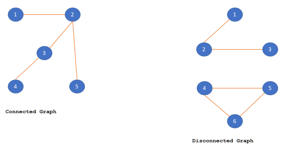
To formalize this idea, let's watch a short video that defines connected components, which it calls "provinces."

The Algorithm: A Systematic Search

So, how do we programmatically find these components? The traversals we learned, DFS and BFS, are the perfect tools. A single call to DFS(start_node) or BFS(start_node) will find all nodes in the component that start_node belongs to. The problem is, it won't find any nodes outside of that component.

The solution is surprisingly simple: we just need to make sure we visit every node in the graph. The algorithm is as follows:

1. Initialize: Create a visited array (or set) for all vertices, initialized to false. Also, initialize a count of components to 0.
2. Iterate: Loop through every vertex v from 0 to V-1.
3. Check and Traverse: Inside the loop, check if vertex v has been visited.
   • If visited[v] is false, it means we have found a new, unexplored component.
   • Increment the component count.
   • Start a traversal (either DFS or BFS) from vertex v. This traversal will explore all nodes in this component and mark them as visited.
4. Finish: Once the loop is complete, count will hold the total number of connected components.

This approach guarantees that we explore the entire graph, one component at a time. Each time our main loop finds an unvisited node, it signifies the start of a new component.

The following video segment masterfully explains and animates this exact logic.

Implementation with DFS and BFS

The beauty of this algorithm is its flexibility. You can use either DFS or BFS as your traversal workhorse; the main looping structure remains the same. Since you are comfortable with Python, let's look at how to implement this.

The article from GeeksforGeeks provides clear, concise Python implementations for finding connected components using both traversal methods.

Let's break down the Python code for the DFS version from the article:

# The main function that finds and returns all connected components
def getComponents(adj):
    V = len(adj)
    visited = [False] * V
    res = [] # A list to store all our components




    # The main loop that iterates through all vertices
    for i in range(V):



        # If a vertex hasn't been visited, it's the start of a new component
        if not visited[i]:
            component = [] # Start a new list for this component



            # Call DFS to find all nodes in this component
            dfs(adj, visited, i, component)
            res.append(component)

    return res




# The standard recursive DFS helper function
def dfs(adj, visited, s, res):
    visited[s] = True
    res.append(s)




    # Recursively visit all adjacent vertices that are not visited
    for i in adj[s]:
        if not visited[i]:
            dfs(adj, visited, i, res)

The BFS version follows the exact same pattern, simply swapping the dfs helper with a bfs helper that uses a queue. This modularity is a powerful concept in algorithm design.

Complexity Analysis

Understanding the performance of this algorithm is crucial. At first glance, a loop running $V$ times that calls a traversal function which runs in $O(V+E)$ might seem to lead to a complexity of $O(V\cdot (V+E))$. However, this is incorrect.

The key is that the traversal function (DFS or BFS) is only ever called on an unvisited node. Once a node is visited, it's marked, and the main loop will skip it. Therefore, each vertex is processed by the main loop's if statement once, and each vertex and edge is visited by one of the traversal calls exactly once over the entire execution of the algorithm.

• Time Complexity: $O(V+E)$

  • The outer loop runs $V$ times.
  • The traversal calls (summed up across all components) visit every vertex and every edge once.
  • Thus, the total time is proportional to $V$ (for the loop checks) + $V+E$ (for all traversals combined), which simplifies to $O(V+E)$.

• Space Complexity: $O(V)$

  • We need a visited array of size $V$.
  • The recursion stack for DFS or the queue for BFS can, in the worst case (a single component that is a long chain), hold up to $O(V)$ vertices.

The video segment below offers a great verbal walkthrough of this time complexity analysis.

Conclusion

Today, we've taken a significant step from basic traversal to practical graph analysis. By wrapping our DFS or BFS algorithms in a simple iterative loop, we've created a powerful tool to decompose a graph into its fundamental connected components.

Here are the key takeaways from this lesson:

• Connected components are disjoint subgraphs where all nodes within a component are mutually reachable.
• The algorithm to find them involves iterating through all vertices and launching a DFS or BFS traversal from any node that has not yet been visited.
• A visited array is essential to keep track of explored nodes across the entire graph, preventing redundant work.
• The number of times a new traversal is started corresponds to the number of connected components.
• Despite the nested structure, the overall time complexity is an efficient $O(V+E)$ because each node and edge is processed only once.

In our next lesson, we will apply our traversal knowledge to another classic problem: finding the shortest path between two nodes in an unweighted graph, for which BFS is uniquely suited.