Choosing and Using Central Tendency Measures

1. What is Central Tendency?

Let's begin by building an intuition for why we need to find the "center" of a dataset. The following video provides an excellent, engaging overview of the three primary ways we measure this: the mean, the median, and the mode.

As the video explained, measures of central tendency give us a single value to summarize a distribution of data. Each one—mean, median, and mode—has its own strengths and weaknesses.

• The mean is the arithmetic average.
• The median is the middle value of an ordered dataset.
• The mode is the most frequently occurring value.

Now, let's formalize these definitions and see how they are applied in a chemical context.

2. Calculating and Applying Measures of Central Tendency

For a more formal look at these calculations, especially as they appear in scientific literature, we'll turn to a resource written for chemists. The following reading uses a very practical example: analyzing the mass of a set of pennies. This is analogous to many common tasks in an analytical lab, like weighing replicate samples.

This reading highlights a critical point: the mean is heavily influenced by outliers (extreme values), while the median is not. This "robustness" makes the median a very reliable measure when your experimental data might contain unusually high or low values, which can happen due to measurement error, sample contamination, or other unforeseen issues.

The chemistry textbook didn't cover the mode in detail, so let's explore it now. The mode is particularly useful for certain types of data.

3. Choosing the Right Measure: It Depends on the Distribution

You now know how to calculate all three measures. The most important skill, however, is knowing which one to use. The choice almost always depends on the distribution of your data—that is, the shape you see when you plot the frequency of your values.

Symmetric vs. Skewed Distributions

• In a symmetric distribution, the data are evenly balanced around the center. A classic example is the "bell curve" or normal distribution, which we will study in depth later.
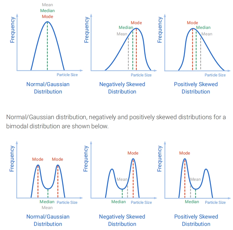
• In a skewed distribution, one tail is longer than the other.
  • Positively skewed (or right-skewed): The long tail is on the right side (higher values). This is common in measurements that cannot be negative, like impurity concentrations or particle sizes.
  • Negatively skewed (or left-skewed): The long tail is on the left side (lower values). This might occur in data like the percent purity of a product, where most batches are close to 100% but some are significantly lower.

The key insight is that the mean is always pulled in the direction of the long tail in a skewed distribution. The median, being the middle point, is not. The following reading illustrates this beautifully.

The image below provides a perfect summary. It shows the relative positions of the mean, median, and mode for various distribution shapes, using "Particle Size" as a variable—a concept highly relevant to your work in materials chemistry.

Guidelines for Selection

Here is a summary to guide your choice:

• Use the Mean when:

  • Your data is numerical (continuous).
  • The distribution is symmetric and doesn't have significant outliers.
  • Example: Replicate measurements of a standard solution's concentration from a well-calibrated instrument.

• Use the Median when:

  • Your data is numerical (continuous or ordinal).
  • The distribution is skewed or contains outliers.
  • Example: Measuring the size of nanoparticles in a sample where a few large agglomerates are present. The mean would be skewed high by the agglomerates, but the median would better represent the size of the primary particles.

• Use the Mode when:

  • You have categorical data.
  • You want to find the most frequent value in a discrete or continuous dataset.
  • Example: You are synthesizing a material and observe several types of crystal habits (e.g., "needle", "plate", "cubic"). The mode tells you which habit is most common. If your distribution has two distinct peaks (bimodal), such as in the particle size data if there are two distinct populations of particles, reporting both modes is more informative than a single mean or median.

Conclusion

In this lesson, we laid the very first stone in our foundation of statistical analysis. You learned how to calculate and, more importantly, how to select and interpret the three measures of central tendency.

Key Takeaways:

• Mean, median, and mode are all single-value summaries of a dataset, but they describe the "center" in different ways.
• The mean is the average, but it is sensitive to outliers and skewed data.
• The median is the middle value and is robust, making it the preferred choice for skewed distributions.
• The mode is the most frequent value and is the only measure applicable to categorical data.
• Choosing the appropriate measure requires you to first consider the distribution and type of your data. A quick visual plot (like a histogram, which we'll cover soon) is often the best first step.

In our next lesson, we will address the other side of the coin: once we know the center of our data, how do we describe its spread or variability? We will explore measures of dispersion, such as range, variance, and standard deviation, to quantify the precision of your experimental results.