Building a 4-bit Ripple-Carry Adder

1. The Concept: Chaining Full Adders

To add two 4-bit numbers, say A[3:0] and B[3:0], we need to perform an addition for each bit position, just like you do with long addition on paper. For each position, we add the corresponding bits A[i] and B[i], plus any carry that came from the position before it. A full adder is perfect for this.

We can build a 4-bit adder by connecting four full adders in a chain. This structure is called a ripple-carry adder.

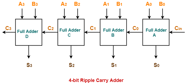
As the diagram shows:

• The first full adder (for the least significant bit, LSB) adds $A[0]$, $B[0]$, and an initial carry-in, $C_{in}$. This $C_{in}$ is usually set to 0 for simple addition.
• The carry-out from this first stage becomes the carry-in for the second full adder, which adds $A[1]$, $B[1]$, and this new carry.
• This process continues, with the carry "rippling" from one stage to the next, until the final full adder calculates the most significant bit (MSB) of the sum and the final carry-out of the entire 4-bit addition.

To see this in action, the following video provides a clear walkthrough of the structure and a practical example.

2. The "Ripple" and Its Consequences: Propagation Delay

The name "ripple-carry adder" points to its most important characteristic and its main limitation. The final sum isn't available instantly. Why? Because the third full adder can't compute its correct result until it receives the carry from the second, which in turn must wait for the carry from the first.

This chain reaction of carries creates a propagation delay. The total time it takes for the circuit to produce a stable, correct output depends on the time it takes for the carry to ripple all the way from the LSB to the MSB.

The next segment of the video you just watched explains this critical concept of propagation delay.

This concept is crucial in real-world chip design. The speed of an adder can directly impact the maximum clock frequency (and thus the performance) of a processor. While a ripple-carry adder is simple, its delay makes it too slow for many high-performance applications. More advanced adders, like carry-lookahead adders, are designed specifically to overcome this delay.

3. Practical Construction in Verilog

Now let's translate the block diagram into Verilog. This aligns with your goal of learning RTL design and your preference for practical application. We will use structural Verilog, where we describe a circuit by instantiating and connecting its sub-components (modules).

This process involves two steps:

1. Defining the building block: a fulladder module.
2. Defining the main module (ripplecarryadder_4bit) and creating four instances of the fulladder inside it, connecting them just like in the diagram.

The following reading provides the complete Verilog code for this.

Let's break down the most important part of the ripplecarryadder_4bit module: the instantiations.

module ripplecarryadder_4bit(sum, cout, a, b, cin);
    output [3:0] sum;
    output       cout;
    input  [3:0] a, b;
    input        cin;
    
    // Internal wires to connect the carry between stages
    wire c0, c1, c2;

    // FA0: Adds the least significant bits (LSB)
    // Takes external cin, produces sum[0] and the first internal carry c0.
    fulladder FA0(sum[0], c0, a[0], b[0], cin);

    // FA1: Adds the next bits
    // Takes carry c0 from FA0, produces sum[1] and internal carry c1.
    fulladder FA1(sum[1], c1, a[1], b[1], c0);

    // FA2: Adds the third bits
    // Takes carry c1 from FA1, produces sum[2] and internal carry c2.
    fulladder FA2(sum[2], c2, a[2], b[2], c1);

    // FA3: Adds the most significant bits (MSB)
    // Takes carry c2 from FA2, produces sum[3] and the final external cout.
    fulladder FA3(sum[3], cout, a[3], b[3], c2);
    
endmodule

Notice how the output port for the carry of one instance (e.g., c0 from FA0) is connected to the input port for the carry of the next instance (c0 into FA1). This is the "cascading" or "rippling" implemented in code. The signals c0, c1, and c2 are declared as wire because they are simply used to connect the modules internally.

Conclusion

In this lesson, we successfully constructed a 4-bit ripple-carry adder, scaling up from the single-bit full adder. This demonstrates a fundamental principle of digital design: building complex functionality from simple, reusable blocks.

Here are the key takeaways:

• A multi-bit ripple-carry adder is built by cascading or chaining several 1-bit full adders.
• The carry-out ($C_{out}$) of each full adder becomes the carry-in ($C_{in}$) for the next, more significant stage.
• This structure leads to propagation delay, as the carry signal must "ripple" through the entire chain before the final result is stable.
• In Verilog, this is implemented using structural modeling, where you instantiate modules and connect their ports with wires.

So far, all the circuits we've built—decoders, multiplexers, and now adders—are combinational. Their outputs depend solely on their current inputs. If you change the input, the output changes (after a propagation delay). They have no memory of past inputs.

In our next lesson, we will begin exploring sequential logic, the other major class of digital circuits. These circuits introduce the concept of state and memory, allowing us to build registers, counters, and ultimately, the complex systems that make up modern processors. We'll start by understanding the role of a clock signal and the fundamental memory element: the flip-flop.