Amortized Analysis of Data Structures

1. The Motivation: Why Worst-Case Isn't Always Enough

Consider a dynamic array, the data structure that backs common list implementations in many languages. You can keep adding elements to it, and it seems to just work. But what happens under the hood when the underlying fixed-size array runs out of space?

A common strategy is to allocate a new, larger array (often double the size), copy all the old elements over, and then add the new element.

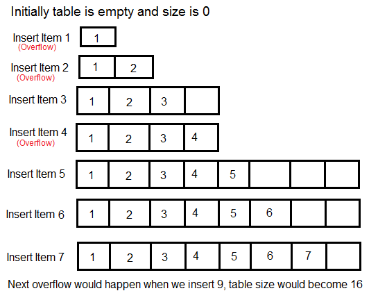
Let's analyze the append operation:

• Best Case: If the array has free space, the operation is O(1). We just place the element in the next available slot.
• Worst Case: If the array is full, we must perform a resize. This involves allocating a new array and copying $n$ elements, making the operation O($n$).

If we only considered the worst case, we might conclude that append is an expensive O($n$) operation. This feels wrong, as we know these data structures are highly performant in practice. The key insight is that the expensive O($n$) operation cannot happen frequently. After a resize, many cheap O(1) operations are guaranteed to follow. Amortized analysis provides the framework to formalize this intuition.

2. Amortized Analysis vs. Average-Case Analysis

Before we proceed, it's critical to distinguish amortized analysis from average-case analysis.

• Average-Case Analysis deals with probability. It requires assumptions about the distribution of inputs (e.g., assuming all possible inputs are equally likely) to calculate an expected running time. If your real-world inputs don't match these assumptions, the analysis may not hold.
• Amortized Analysis does not involve probability. It provides a worst-case guarantee for a sequence of operations. It proves that the average cost per operation, over any possible sequence, will not exceed a certain bound.

For interview preparation, this distinction is vital. Amortized analysis gives a deterministic guarantee, which is a much stronger claim.

To start building a solid foundation, let's explore the core ideas and the three main methods of amortized analysis.

Now that you have the conceptual background, let's dive into the three main techniques for performing amortized analysis. We'll use the dynamic array with a doubling strategy as our case study for all three.

3. Method 1: The Aggregate Method

This is the most straightforward approach. The logic is simple:

1. Calculate the total worst-case cost, $T(n)$, for a sequence of $n$ operations.
2. The amortized cost per operation is then $T(n)/n$.

Let's apply this to a sequence of $n$ append operations on an initially empty dynamic array. We'll use a simple cost model where inserting an element costs 1 unit and copying an element during a resize also costs 1 unit.

To see this in action, this video provides a great visual and mathematical breakdown.

As the video shows, for a sequence of $n$ insertions:

• Insertion Costs: There are $n$ insertions, each costing 1. Total = $n$.
• Copying Costs: Resizing happens at sizes 1, 2, 4, 8, ..., up to the largest power of 2 less than $n$. The total copy cost is the sum $1+2+4+\cdots +2^k$ where $2^k<n$. This geometric series sums to $2^{k+1}-1$, which is less than $2n$.
• Total Cost: The total cost is at most $n$ (for insertions) + $2n$ (for copying) = $3n$.
• Amortized Cost: The total cost for $n$ operations is O($n$). Therefore, the amortized cost per operation is O($n$) / $n$ = O(1).

4. Method 2: The Accounting (or Banker's) Method

This method uses a simple and powerful analogy. Imagine you are "charging" each operation a fixed amount, called the amortized cost.

• If an operation's actual cost is less than its charge, the difference is saved as "credit."
• This credit is stored with the data structure (e.g., with the elements themselves).
• If an operation's actual cost is more than its charge, it can use the saved credit to pay for the extra work.

The key is to set a charge high enough that the "bank balance" of credit never goes negative.

Let's watch how this is applied to our dynamic array.

Here's a summary of the logic for the dynamic array:

• Set the amortized cost (charge) to 3 units for every append.
• When an element is appended without a resize:
  • Actual cost is 1 unit (for the insertion).
  • We use 1 unit of the charge to pay for it.
  • The remaining 2 units are stored as credit with the newly inserted element.
• When a resize is triggered at size $n$:
  • The array is full. The last $n/2$ elements were added since the previous resize.
  • Each of these $n/2$ elements has 2 units of credit stored. Total credit available = $(n/2)\times 2=n$.
  • The cost to copy the $n$ old elements is exactly $n$.
  • We use the stored credit to pay for the copy. The cost of the resize itself becomes 0 from an amortized perspective!
  • The new element being added still pays its 3 units. 1 for its own insertion, and 2 are stored as credit.

Since we can always pay for the expensive resizes with saved credit, the cost for any operation is bounded by the constant charge of 3. Thus, the amortized cost is O(1).

5. Method 3: The Potential Method (Physicist's Method)

This is the most formal and versatile method. It's analogous to potential energy in physics. We define a potential function, $\Phi$, which maps the state of the data structure to a number representing the stored "potential."

The amortized cost of an operation is defined as:

where $\Delta \Phi$ is the change in potential (${\Phi }_{after}-{\Phi }_{before}$).

• Cheap operations should increase the potential ($\Delta \Phi >0$), making their amortized cost higher than their actual cost.
• Expensive operations should decrease the potential ($\Delta \Phi <0$), using the stored potential to "pay for" the work, making their amortized cost lower than their actual cost.

The main challenge is choosing a suitable potential function, $\Phi$. For the function to be valid, we typically require $\Phi (D_0)=0$ (for the initial state $D_0$) and $\Phi (D_i)\ge 0$ for all subsequent states $D_i$.

For our dynamic array with $n$ elements and capacity $c$, a good potential function is:

Let's see why this works.

Let's re-examine the two cases using this potential function:

Case 1: No resize ($n<c$)

• Actual cost = 1.
• Before: $n_{before}=n$, $c_{before}=c$. ${\Phi }_{before}=2n-c$.
• After: $n_{after}=n+1$, $c_{after}=c$. ${\Phi }_{after}=2(n+1)-c=2n-c+2$.
• $\Delta \Phi ={\Phi }_{after}-{\Phi }_{before}=2$.
• Amortized cost = Actual cost + $\Delta \Phi =1+2=3$.

Case 2: Resize ($n=c$)

• Actual cost = $n+1$ (to copy $n$ items and insert the new one).
• Before: $n_{before}=n$, $c_{before}=n$. ${\Phi }_{before}=2n-n=n$.
• After: $n_{after}=n+1$, $c_{after}=2n$. ${\Phi }_{after}=2(n+1)-2n=2n+2-2n=2$.
• $\Delta \Phi ={\Phi }_{after}-{\Phi }_{before}=2-n$.
• Amortized cost = Actual cost + $\Delta \Phi =(n+1)+(2-n)=3$.

In both cases, the amortized cost is 3. Since the amortized cost is constant for every operation, we conclude the performance is O(1). The art and power of this method lie in finding the right potential function, which is a skill that comes with practice.

For a more rigorous exploration of how one arrives at a potential function, I highly recommend reviewing the CMU notes again, this time focusing on the potential method section.

Conclusion

Today you've added a crucial tool to your analytical toolkit. While worst-case analysis of a single operation is important, amortized analysis provides a more accurate picture for data structures where costs are spread out over a sequence of operations.

Key Takeaways:

• Amortized analysis calculates the average cost of an operation over a sequence in the worst case, without using probabilities.
• It's ideal for structures with infrequent, expensive "cleanup" or "rebuilding" operations, like a dynamic array's resize.
• Aggregate Method: Simple but effective. Total cost over $n$ operations divided by $n$.
• Accounting Method: Intuitive "banking" analogy. Overcharge cheap operations to save credit for expensive ones.
• Potential Method: The most formal method. Uses a potential function to model "pre-paid work" stored in the data structure. The amortized cost is the actual cost plus the change in potential.
• For a dynamic array using a doubling strategy, the append operation has a worst-case time of O($n$) but an amortized time of O(1).

In our next lesson, we will shift gears from pure analysis back to implementation. We will start building our foundational problem-solving skills by tackling simple recursive problems. Mastering recursion is the bedrock for approaching more complex topics like tree traversals, backtracking, and dynamic programming, which are cornerstones of technical interviews.