Master Theorem for Recurrence Relations

1. The Anatomy of a Divide-and-Conquer Recurrence

The Master Theorem applies to recurrence relations of the form:

$T(n)=aT(n/b)+f(n)$

where:

• $n$ is the size of the problem.
• $a$ is the number of subproblems in the recursion. It must be greater than or equal to 1 ($a\ge 1$).
• $n/b$ is the size of each subproblem. Here, $b$ is the factor by which the problem size is reduced. It must be greater than 1 ($b>1$).
• $f(n)$ is the cost of the work done outside the recursive calls. This includes the time spent dividing the problem and the time spent combining the solutions from the subproblems.

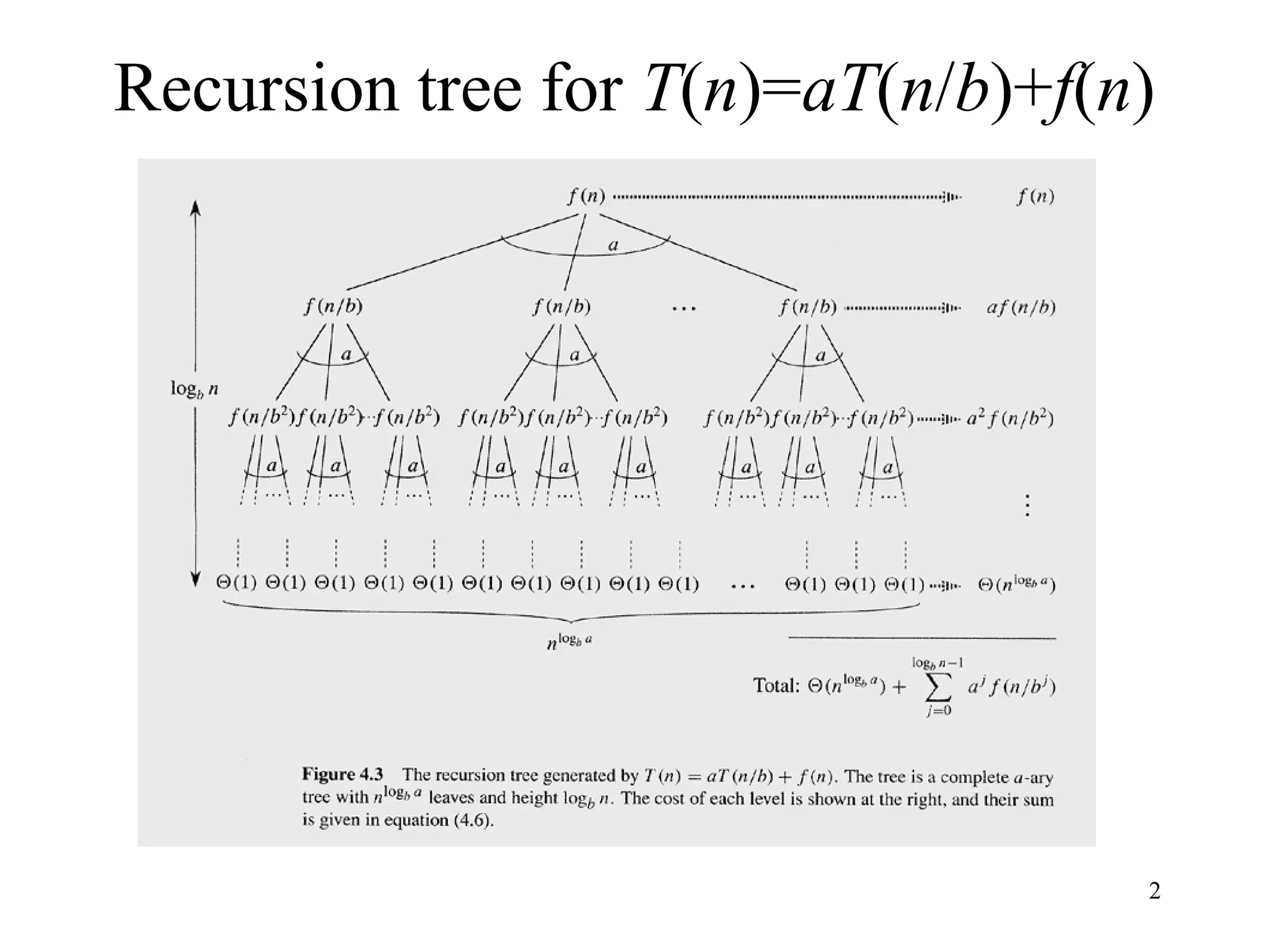
Let's use Merge Sort as a concrete example: $T(n)=2T(n/2)+n$.

• $a=2$: We divide the array into two subproblems (the left and right halves).
• $b=2$: Each subproblem is half the size of the original.
• $f(n)=\Theta (n)$: The merge step takes linear time to combine the two sorted halves.

2. The Intuition: A Competition of Forces

The Master Theorem is essentially a way to determine which part of the recurrence dominates the overall complexity. Think of it as a competition between two forces:

1. The Recursive Part: The term $aT(n/b)$ represents the cost of solving the subproblems. The growth of this part is determined by the "watershed function" $n^{{\log }_{b}a}$. This value intuitively represents the number of leaves in the recursion tree, signifying the total number of base-case subproblems we end up with.
2. The Work-per-Level Part: The term $f(n)$ represents the work done at each level of recursion (to divide and combine).

The Master Theorem simply compares the growth rate of $f(n)$ to the growth rate of $n^{{\log }_{b}a}$ and tells you which one dictates the final complexity.

To build a strong mental model for this, I recommend reading the following short document. It offers a clear, high-level intuition before we dive into the formal cases.

This intuition is also visualized well on the VisuAlgo site. In their terminology, they compare the "driving function" $g(n)$ (our $f(n)$) with the "watershed function" $n^{{\log }_{b}a}$. The cost at each level of the recursion tree either grows, stays the same, or shrinks, which directly corresponds to the three cases of the theorem.

3. The Three Cases of the Master Theorem

The theorem compares $f(n)$ with $n^{{\log }_{b}a}$. For simplicity in most common interview problems, we often assume $f(n)$ is of the form $n^c$. The comparison then boils down to comparing the exponents: ${\log }_{b}a$ vs. $c$.

Let's look at the three cases that arise from this comparison.

Case 1: The Recursion Dominates

• Condition: If $n^{{\log }_{b}a}$ grows polynomially faster than $f(n)$. Formally, if $f(n)=O(n^{{\log }_{b}a-ϵ})$ for some constant $ϵ>0$.
  • Simple check: If $f(n)=\Theta (n^c)$, this case applies when ${\log }_{b}a>c$.
• Result: The complexity is dominated by the number of leaves in the recursion tree.
  • $T(n)=\Theta (n^{{\log }_{b}a})$

Example: Strassen's Matrix Multiplication: $T(n)=7T(n/2)+\Theta (n^2)$.

• $a=7,b=2,f(n)=\Theta (n^2)$ so $c=2$.
• Calculate ${\log }_{b}a={\log }_{2}7\approx 2.81$.
• Since $2.81>2$, Case 1 applies.
• The result is $T(n)=\Theta (n^{{\log }_{2}7})$.

Case 2: The Work is Balanced

• Condition: If $n^{{\log }_{b}a}$ and $f(n)$ grow at roughly the same rate. Formally, if $f(n)=\Theta (n^{{\log }_{b}a}{\log }^{k}n)$ for some constant $k\ge 0$.
  • Simple check: If $f(n)=\Theta (n^c)$ (i.e., $k=0$), this case applies when ${\log }_{b}a=c$.
• Result: The work at each level is comparable, so we multiply by the number of levels, which is logarithmic.
  • $T(n)=\Theta (n^{{\log }_{b}a}{\log }^{k+1}n)$
  • For the simple case where $k=0$, this is $T(n)=\Theta (n^c\log n)$.

Example: Merge Sort: $T(n)=2T(n/2)+\Theta (n)$.

• $a=2,b=2,f(n)=\Theta (n)$ so $c=1$.
• Calculate ${\log }_{b}a={\log }_{2}2=1$.
• Since $1=1$, Case 2 applies (with $k=0$).
• The result is $T(n)=\Theta (n^1\log n)=\Theta (n\log n)$.

Case 3: The Combination Work Dominates

• Condition: If $f(n)$ grows polynomially faster than $n^{{\log }_{b}a}$. Formally, if $f(n)=\Omega (n^{{\log }_{b}a+ϵ})$ for some constant $ϵ>0$.
  • Simple check: If $f(n)=\Theta (n^c)$, this case applies when ${\log }_{b}a<c$.
• Additional Condition (Regularity): For this case to hold, you must also satisfy the condition that $af(n/b)\le Cf(n)$ for some constant $C<1$ and sufficiently large $n$. This condition is a technicality ensuring that the work at the root is indeed the dominant part. For polynomial $f(n)$, it's almost always satisfied.
• Result: The complexity is dominated by the work done at the top level of the recursion.
  • $T(n)=\Theta (f(n))$

Example: A fictional recurrence $T(n)=3T(n/4)+\Theta (n\log n)$.

• $a=3,b=4,f(n)=\Theta (n\log n)$. For the simple check, we approximate $f(n)$ as being "stronger" than $n^1$, so we check against $c=1$.
• Calculate ${\log }_{b}a={\log }_{4}3\approx 0.79$.
• Since $0.79<1$, Case 3 applies. The regularity condition holds as well.
• The result is $T(n)=\Theta (f(n))=\Theta (n\log n)$.

4. Practical Application: Seeing the Patterns

Now that you have the theory, let's focus on applying it quickly and accurately. The following video by Abdul Bari is excellent for this. He uses a slightly different notation (k instead of c, p for the log exponent) but the logic is identical and his rapid-fire examples are perfect for building pattern-recognition skills.

Now, let's solidify your understanding by working through the systematic examples from the UMD lecture notes.

5. Deeper Dive: Formal Definitions and Limitations

Your goal is to build a deep foundation, so it's worth seeing the more rigorous definitions used in formal computer science literature (like the CLRS textbook). The video below uses these more formal definitions involving $ϵ$ and Big Omega/Theta notation. You don't need to memorize these for most interviews, but understanding them clarifies why the simpler comparison works.

It's also important to know when the Master Theorem does not apply:

• The recurrence is not in the form $aT(n/b)+f(n)$. Example: $T(n)=T(n/2)+T(n/3)+n$.
• The function $f(n)$ is not polynomially bounded. Example: $T(n)=2T(n/2)+n!$.
• The gap between $f(n)$ and $n^{{\log }_{b}a}$ is not polynomial. Example: $T(n)=2T(n/2)+n\log n$. This falls into a gap between cases in some simplified versions of the theorem, but is handled by the extended Case 2 we saw earlier ($k=1$).

Conclusion

You've now learned one of the most practical tools for algorithmic analysis. The Master Theorem provides a powerful shortcut to solve recurrence relations for divide-and-conquer algorithms, which are common in both theory and practice.

Key Takeaways:

• The Master Theorem solves recurrences of the form $T(n)=aT(n/b)+f(n)$.
• The analysis boils down to a competition between the work from recursion ($n^{{\log }_{b}a}$) and the work done at each step ($f(n)$).
• Case 1 (${\log }_{b}a>c$): The recursion dominates. $T(n)=\Theta (n^{{\log }_{b}a})$.
• Case 2 (${\log }_{b}a=c$): The work is balanced. $T(n)=\Theta (n^c\log n)$.
• Case 3 (${\log }_{b}a<c$): The non-recursive work dominates. $T(n)=\Theta (f(n))$.
• Being able to quickly identify a, b, and f(n) and apply the correct case is a key interview skill.

In our next lesson, we will explore Amortized Analysis. This is another essential analysis technique, but it takes a different perspective. Instead of analyzing a single operation in the worst-case, it analyzes the average cost of operations over a sequence, which is crucial for understanding data structures like dynamic arrays or hash tables where occasional expensive operations are "paid for" by many cheap ones.